
Dummy list paragraph
Calc Guide
Chapter
1
Introducing Calc
Using Spreadsheets in LibreOffice
This document is Copyright © 2005–2011 by its contributors as listed below. You may distribute it and/or modify it under the terms of either the GNU General Public License (http://www.gnu.org/licenses/gpl.html), version 3 or later, or the Creative Commons Attribution License (http://creativecommons.org/licenses/by/3.0/), version 3.0 or later.
All trademarks within this guide belong to their legitimate owners.
Contributors
Barbara Duprey
Hal Parker
Feedback
Please direct any comments or suggestions about this document to: documentation@libreoffice.org
Acknowledgments
This chapter is based on Chapter 1 of the OpenOffice.org 3.3 Calc Guide. The contributors to that chapter are:
Rick Barnes Nicole Cairns
Peter
Kupfer Jean Hollis Weber
Krishna Aradhi Andy Brown
Alexandre
Martins Anthony Petrillo
Gary Schnabl Barbara M Tobias
Publication date and software version
Published 29 April 2011. Based on LibreOffice 3.3.2.
Some keystrokes and menu items are different on a Mac from those used in Windows and Linux. The table below gives some common substitutions for the instructions in this chapter. For a more detailed list, see the application Help.
|
Windows/Linux |
Mac equivalent |
Effect |
|
Tools → Options menu selection |
LibreOffice → Preferences |
Access setup options |
|
Right-click |
Control+click |
Open context menu |
|
Ctrl (Control) |
z (Command) |
Used with other keys |
|
F5 |
Shift+z+F5 |
Open the Navigator |
|
F11 |
z+T |
Open Styles & Formatting window |
Contents
Spreadsheets, sheets, and cells 5
Parts of the main Calc window 5
Right-click (context) menus 10
Starting a new document from a template 14
Opening existing spreadsheets 14
Saving a document automatically 16
Saving as a Microsoft Excel document 16
Navigating within spreadsheets 20
Selecting items in a sheet or spreadsheet 23
Working with columns and rows 25
Calc is the spreadsheet component of LibreOffice. You can enter data (usually numerical) in a spreadsheet and then manipulate this data to produce certain results.
Alternatively, you can enter data and then use Calc in a ‘What if...’ manner by changing some of the data and observing the results without having to retype the entire spreadsheet or sheet.
Other features provided by Calc include:
Functions, which can be used to create formulas to perform complex calculations on data
Database functions, to arrange, store, and filter data
Dynamic charts; a wide range of 2D and 3D charts
Macros, for recording and executing repetitive tasks; scripting languages supported include LibreOffice Basic, Python, BeanShell, and JavaScript
Ability to open, edit, and save Microsoft Excel spreadsheets
Import and export of spreadsheets in multiple formats, including HTML, CSV, PDF, and PostScript
|
Note |
If you want to use macros written in Microsoft Excel using the VBA macro code in LibreOffice, you must first edit the code in the LibreOffice Basic IDE editor. See Chapter 12, Calc Macros. |
Spreadsheets, sheets, and cells
Calc works with elements called spreadsheets. Spreadsheets consist of a number of individual sheets, each sheet containing cells arranged in rows and columns. A particular cell is identified by its row number and column letter.
Cells hold the individual elements—text, numbers, formulas, and so on—that make up the data to display and manipulate.
Each spreadsheet can have many sheets, and each sheet can have many individual cells. In Calc 3.3, each sheet can have a maximum of 1,048,576 (65,536 rows in Calc 3.2 and earlier) and a maximum of 1024 columns
When Calc is started, the main window looks similar to Figure 1.
|
Note |
If any part of the Calc window in Figure 1 is not shown, you can display it using the View menu. For example, View → Status Bar will toggle (show or hide) the Status Bar. It is not always necessary to display all the parts, as shown; show or hide any of them, as desired. |
The Title bar, located at the top, shows the name of the current spreadsheet. When the spreadsheet is newly created, its name is Untitled X, where X is a number. When you save a spreadsheet for the first time, you are prompted to enter a name of your choice.
Under the Title bar is the Menu bar. When you choose one of the menus, a submenu appears with other options. You can modify the Menu bar, as discussed in Chapter 14, Setting Up and Customizing Calc.
File contains commands that apply to the entire document such as Open, Save, Wizards, Export as PDF, and Digital Signatures.
Edit contains commands for editing the document such as Undo, Changes, Compare Document, and Find and Replace.
View contains commands for modifying how the Calc user interface looks such as Toolbars, Full Screen, and Zoom.
Insert contains commands for inserting elements such as cells, rows, columns, sheets, and pictures into a spreadsheet.
Format contains commands for modifying the layout of a spreadsheet such as Styles and Formatting, Paragraph, and Merge Cells.
Tools contains functions such as Spelling, Share Document, Cell Contents, Gallery, and Macros.
Data contains commands for manipulating data in your spreadsheet such as Define Range, Sort, Filter, and DataPilot.
Window contains commands for the display window such as New Window, Split, and Freeze.
Help contains links to the Help file bundled with the software, What's This?, Support, Registration, and Check for Updates.
Calc has several types of toolbars: docked (fixed in place), floating, and tear-off. Docked toolbars can be moved to different locations or made to float, and floating toolbars can be docked.
Four toolbars are located under the Menu bar by default: the Standard toolbar, the Find toolbar, the Formatting toolbar, and the Formula Bar.
The icons (buttons) on these toolbars provide a wide range of common commands and functions. You can also modify these toolbars, as discussed in Chapter 14, Setting Up and Customizing Calc.
Placing the mouse pointer over any of the icons displays a small box, called a tooltip. It gives a brief explanation of the icon’s function. For a more detailed explanation, choose Help → What’s This? and hover the mouse pointer over the icon. To turn this feature off again, click once or press the Esc key twice. Tips and extended tips can be turned on or off from Tools → Options → LibreOffice → General.
Displaying or hiding toolbars
To display or hide toolbars, choose View → Toolbars, then click on the name of a toolbar in the list. An active toolbar shows a check mark beside its name. Tear-off toolbars are not listed in the View menu.
Palettes and tear-off toolbars
Toolbar icons with a small triangle to the right will display palettes, tear-off toolbars, and other ways of selecting things, depending on the icon.
An example of a palette is shown in Figure 2. It is displayed by clicking the small triangle to the right of the Borders toolbar icon.
An example of a tear-off toolbar is shown in Figure 3. Tear-off toolbars can be floating or docked along an edge of the screen or in one of the existing toolbar areas. To move a floating tear-off toolbar, drag it by the title bar.
To move a docked toolbar, place the mouse pointer over the toolbar handle, hold down the left mouse button, drag the toolbar to the new location, and then release the mouse button.
To move a floating toolbar, click on its title bar and drag it to a new location, as shown in Figure 3.
Docking/floating windows and toolbars
Toolbars and some windows, such as the Navigator and the Styles and Formatting window, are dockable. You can move, resize, or dock them to an edge.
To dock a window or toolbar, hold down the Control key and double-click on the frame of the floating window (or in a vacant area near the icons at the top of the floating window) to dock it in its last position.
To undock a window, hold down the Control key and double-click on the frame (or a vacant area near the icons at the top) of the docked window.
You can customize toolbars in several ways, including choosing which icons are visible and locking the position of a docked toolbar.
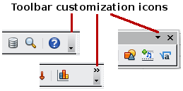
To
access a toolbar’s customization options, use the down-arrow at the
end of the toolbar or on its title bar.
To show or hide icons defined for the selected toolbar, choose Visible Buttons from the drop-down menu. Visible icons are indicated by a border around the icon (Figure 6). Click on icons to hide or show them on the toolbar.
You can also add icons and create new toolbars, as described in Chapter 16.
In the Formatting toolbar, the three boxes on the left are the Apply Style, Font Name, and Font Size lists (see Figure 7). They show the current settings for the selected cell or area. (The Apply Style list may not be visible by default.) Click the down-arrow to the right of each box to open the list.
|
Note |
If any of the icons (buttons) in Figure 7 is not shown, you can display it by clicking the small triangle at the right end of the Formatting toolbar, selecting Visible Buttons in the drop-down menu, and selecting the desired icon (for example, Apply Style) in the drop-down list. It is not always necessary to display all the toolbar buttons, as shown; show or hide any of them, as desired. |
On the left hand side of the Formula Bar is a small text box, called the Name Box, with a letter and number combination in it, such as D7. This combination, called the cell reference, is the column letter and row number of the selected cell.
To the right of the Name Box are the Function Wizard, Sum, and Function buttons.
Clicking the Function Wizard button opens a dialog from which you can search through a list of available functions. This can be very useful because it also shows how the functions are formatted.
In a spreadsheet the term function covers much more than just mathematical functions. See Chapter 7, Using Formulas and Functions, for more details.
Clicking the Sum button inserts a formula into the current cell that totals the numbers in the cells above the current cell. If there are no numbers above the current cell, then the cells to the left are placed in the Sum formula.
Clicking the Function button inserts an equals (=) sign into the selected cell and the Input line, thereby enabling the cell to accept a formula.
When
you enter new data into a cell, the Sum and Equals buttons change to
Cancel
and Accept
buttons
![]() .
.
The contents of the current cell (data, formula, or function) are displayed in the Input line, which is the remainder of the Formula Bar. You can either edit the cell contents of the current cell there, or you can do that in the current cell. To edit inside the Input line area, click in the area, then type your changes. To edit within the current cell, just double-click the cell.
Right-click on a cell, graphic, or other object to open a context menu. Often the context menu is the fastest and easiest way to reach a function. If you’re not sure where in the menus or toolbars a function is located, you may be able to find it by right-clicking.
The main section of the screen displays the cells in the form of a grid, with each cell being at the intersection of a column and a row.
At the top of the columns and at the left end of the rows are a series of gray boxes containing letters and numbers. These are the column and row headers. The columns start at A and go on to the right, and the rows start at 1 and go down.
These column and row headers form the cell references that appear in the Name Box on the Formula Bar (see Figure 8). You can turn these headers off by selecting View → Column & Row Headers.
At the bottom of the grid of cells are the sheet tabs. These tabs enable access to each individual sheet, with the visible (active) sheet having a white tab. Clicking on another sheet tab displays that sheet, and its tab turns white. You can also select multiple sheet tabs at once by holding down the Control key while you click the names.
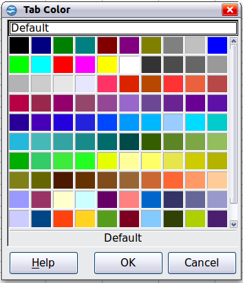
From Calc 3.3, you can choose colors for the different sheet tabs. Right-click on a tab and choose Tab Color from the context menu to open a palette of colors. To add new colors to the palette, see “Color options” in Chapter 14, Setting up and Customizing Calc.
The Calc status bar provides information about the spreadsheet and convenient ways to quickly change some of its features.
Sheet
sequence number (![]() )
)
Shows the sequence number of the current sheet and the total number of sheets in the spreadsheet. The sequence number may not correspond with the name on the sheet tab.
Page
style (![]() )
)
Shows the page style of the current sheet. To edit the page style, double-click on this field. The Page Style dialog opens.
Insert
mode (![]() )
)
Click to toggle between INSRT (Insert) and OVER (Overwrite) modes when typing. This field is blank when the spreadsheet is not in a typing mode (for example, when selecting cells).
Selection
mode (![]() )
)
Click to toggle between STD (Standard), EXT (Extend), and ADD (Add) selection. EXT is an alternative to Shift+click when selecting cells. See page 23 for more information.
Unsaved
changes (![]() )
)
An icon appears here if changes to the spreadsheet have not been saved.
Digital
signature (![]() )
)
If the document has not been digitally signed, double-clicking in this area opens the Digital Signatures dialog, where you can sign the document. See Chapter 6, Printing, Exporting, and E-mailing, for more about digital signatures.
If
the document has been digitally signed, an icon
![]() shows in this area. You can double-click the icon to view the
certificate. A document can be digitally signed only after it has
been saved.
shows in this area. You can double-click the icon to view the
certificate. A document can be digitally signed only after it has
been saved.
Cell or
object information (![]() )
)
Displays information about the selected items. When a group of cells is selected, the sum of the contents is displayed by default; you can right-click on this field and select other functions, such as the average value, maximum value, minimum value, or count (number of items selected).
When the cursor is on an object such as a picture or chart, the information shown includes the size of the object and its location.
To change the view magnification, drag the Zoom slider or click on the + and – signs. You can also right-click on the zoom level percentage to select a magnification value or double-click to open the Zoom & View Layout dialog.
You can start a new, blank document in Calc in several ways.
From the operating system menu, in the same way that you start other programs. When LibreOffice was installed on your computer, in most cases a menu entry for each component was added to your system menu. If you are using a Mac, you should see the LibreOffice icon in the Applications folder. When you double-click this icon, LibreOffice opens at the Start Center (Figure 13).
From the Quickstarter, which is found in Windows, some Linux distributions, and (in a slightly different form) in Mac OS X. The Quickstarter is an icon that is placed in the system tray or the dock during system startup. It indicates that LibreOffice has been loaded and is ready to use.
Right-click the Quickstarter icon (Figure 12) in the system tray to open a menu from which you can open a new document, open the Templates and Documents dialog box, or choose an existing document to open. You can also double-click the Quickstarter icon to display the Templates and Documents dialog box.
See Chapter 1, Introducing LibreOffice, in the Getting Started guide for more information about using the Quickstarter.
From the Start Center. When LibreOffice is open but no document is open (for example, if you close all the open documents but leave the program running), the Start Center is shown. Click one of the icons to open a new document of that type, or click the Templates icon to start a new document using a template. If a document is already open in LibreOffice, the new document opens in a new window.
When LibreOffice is open, you can also start a new document in one of the following ways.
Press the Control+N keys.
Use File → New → Spreadsheet.
Click the New button on the main toolbar.
Starting a new document from a template
Calc documents can also be created from templates. Follow the above procedures, but instead of choosing Spreadsheet, choose the Templates icon from the Start Center or File → New → Templates and Documents from the Menu bar or toolbar.
On the Templates and Documents window (Figure 14), navigate to the appropriate folder and double-click on the required template. A new spreadsheet, based on the selected template, opens.
A new LibreOffice installation does not contain many templates, but you can add more by downloading them from http://extensions.libreoffice.org/ and installing them as described in Chapter 14, Setting Up and Customizing Calc.
When no document is open, the Start Center (Figure 22) provides an icon for opening an existing document or choosing from a list of recently-edited documents.
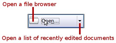
You can also open an existing document in one of the following ways. If a document is already open in LibreOffice, the second document opens in a new window.
Choose File → Open....
Click the Open button on the main toolbar.
Press Control+O on the keyboard.
Use File → Recent Documents to display the last 10 files that were opened in any of the LibreOffice components.
Use the Open Document selection on the Quickstarter.
In each case, the Open dialog box appears. Select the file you want, and then click Open. If a document is already open in LibreOffice, the second document opens in a new window.
If you have associated Microsoft Office file formats with LibreOffice, you can also open these files by double-clicking on them.
Comma-separated-values (CSV) files are text files that contain the cell contents of a single sheet. Each line in a CSV file represents a row in a spreadsheet. Commas, semicolons, or other characters are used to separate the cells. Text is entered in quotation marks; numbers are entered without quotation marks.
To open a CSV file in Calc:
Choose File → Open.
Locate the CSV file that you want to open.
If the file has a *.csv extension, select the file and click Open.
If the file has another extension (for example, *.txt), select the file, select Text CSV (*csv;*txt) in the File type box (scroll down into the spreadsheet section to find it), and then click Open.
On the Text Import dialog (Figure 15), select the Separator options to divide the text in the file into columns.
You can preview the layout of the imported data at the bottom of the dialog. Right-click a column in the preview to set the format or to hide the column.
If the CSV file uses a text delimiter character that is not in the Text delimiter list, click in the box, and type the character.
The choices in the Other options section determine whether quoted data will always be imported as text, and whether Calc will automatically detect all number formats, including special number formats such as dates, time, and scientific notation. The detection depends on the language settings.
Click OK to open the file.
|
Caution
|
If you do not select Text CSV (*csv;*txt) as the file type when opening the file, the document opens in Writer, not Calc. |
Spreadsheets can be saved in three ways.
Press Control+S.
Choose File → Save (or Save All or Save As).
Click the Save button on the main toolbar.
If the spreadsheet has not been saved previously, then each of these actions will open the Save As dialog. There you can specify the spreadsheet name and the location in which to save it.
|
Note |
If the spreadsheet has been previously saved, then saving it using the Save (or Save All) command will overwrite an existing copy. However, you can save the spreadsheet in a different location or with a different name by selecting File → Save As. |
Saving a document automatically
You can choose to have Calc save your spreadsheet automatically at regular intervals. Automatic saving, like manual saving, overwrites the last saved state of the file. To set up automatic file saving:
Choose Tools → Options → Load/Save → General.
Click on Save AutoRecovery information every and set the time interval. The default value is 15 minutes. Enter the value you want by typing it or by pressing the up or down arrow keys.
Saving as a Microsoft Excel document
If you need to exchange files with users of Microsoft Excel, they may not know how to open and save *.ods files. Only Microsoft Excel 2007 with Service Pack 2 (SP2) can do this. Users of Microsoft Excel 2007, 2003, XP, and 2000 can also download and install a free OpenDocument Format (ODF) plugin from Sun Microsystems, available from Softpedia, http://www.softpedia.com/get/Office-tools/Other-Office-Tools/Sun-ODF-Plugin-for-Microsoft-Office.shtml.
Some users of Microsoft Excel may be unwilling or unable to receive *.ods files. (Perhaps their employer does not allow them to install the plug-in.) In this case, you can save a document as a Excel file (*.xls or *.xlsx).
Important—First save your spreadsheet in the file format used by LibreOffice, *.ods. If you do not, any changes you may have made since the last time you saved it will only appear in the Microsoft Excel version of the document.
Then choose File → Save As.
On the Save As dialog (Figure 16), in the File type (or Save as type) drop-down menu, select the type of Excel format you need. Click Save.
|
Caution
|
From this point on, all changes you make to the spreadsheet will occur only in the Microsoft Excel document. You have changed the name and file type of your document. If you want to go back to working with the *.ods version of your spreadsheet, you must open it again. |
|
Tip |
To have Calc save documents by default in a Microsoft Excel file format, go to Tools → Options → Load/Save → General. In the section named Default file format and ODF settings, under Document type, select Spreadsheet, then under Always save as, select your preferred file format. |
To save a spreadsheet as a comma separated value (CSV) file:
Choose File → Save As.
In the File name box, type a name for the file.
In the File type list, select Text CSV (.csv) and click Save.
You may see the message box shown below. Click Keep Current Format.
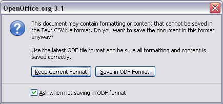
In the Export of text files dialog, select the options you want and then click OK.
Calc can save spreadsheets in a range of formats, including HTML (Web pages), through the Save As dialog. Calc can also export spreadsheets to the PDF and XHTML file formats. See Chapter 6, Printing, Exporting, and E-mailing, for more information.
Calc provides two levels of document protection: read-protect (file cannot be viewed without a password) and write-protect (file can be viewed in read-only mode but cannot be changed without a password). Thus you can make the content available for reading by a selected group of people and for reading and editing by a different group. This behavior is compatible with Microsoft Excel file protection.
Use File → Save As when saving the document. (You can also use File → Save the first time you save a new document.)
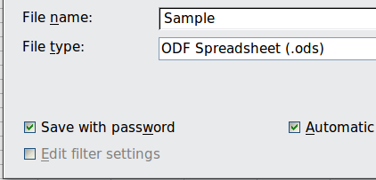
On the Save As dialog, type the file name, select the Save with password option, and then click Save.
The Set Password dialog opens.
Here you have several choices:
To read-protect the document, type a password in the two fields at the top of the dialog box.
To write-protect the document, click the More Options button and select the Open file read-only checkbox.
To write-protect the document but allow selected people to edit it, select the Open file read-only checkbox and type a password in the two boxes at the bottom of the dialog box.
Click OK to save the file. If either pair of passwords do not match, you receive an error message. Close the message box to return to the Set Password dialog box and enter the password again.
|
Caution
|
LibreOffice uses a very strong encryption mechanism that makes it almost impossible to recover the contents of a document if you lose the password. |
Navigating within spreadsheets
Calc provides many ways to navigate within a spreadsheet from cell to cell and sheet to sheet. You can generally use whatever method you prefer.
Using the mouse
Place the mouse pointer over the cell and click.
Using a cell reference
Click on the little inverted black triangle just to the right of the Name Box (Figure 8). The existing cell reference will be highlighted. Type the cell reference of the cell you want to go to and press Enter. Cell references are case insensitive: a3 or A3, for example, are the same. Or just click into the Name Box, backspace over the existing cell reference, and type in the cell reference you want and press Enter.
Using the Navigator
Click on the Navigator button in the Standard toolbar (or press F5) to display the Navigator. Type the cell reference into the top two fields, labeled Column and Row, and press Enter. In Figure 31 on page 32, the Navigator would select cell A7. For more about using the Navigator, see page 31.
In the spreadsheet, one cell normally has a darker black border. This black border indicates where the focus is (see Figure 19). The focus indicates which cell is enabled to receive input. If a group of cells is selected, they have a highlight color (usually gray), with the focus cell having a dark border.
Using the mouse
To move the focus using the mouse, simply move the mouse pointer to the cell where you want the focus to be and click the left mouse button. This action changes the focus to the new cell. This method is most useful when the two cells are a large distance apart.
Using the Tab and Enter keys
Pressing Enter or Shift+Enter moves the focus down or up, respectively.
Pressing Tab or Shift+Tab moves the focus to the right or to the left, respectively.
Using the arrow keys
Pressing the arrow keys on the keyboard moves the focus in the direction of the arrows.
Using Home, End, Page Up and Page Down
Home moves the focus to the start of a row.
End moves the focus to the column furthest to the right that contains data.
Page Down moves the display down one complete screen and Page Up moves the display up one complete screen.
Combinations of Control (often represented on keyboards as Ctrl) and Alt with Home, End, Page Down (PgDn), Page Up (PgUp), and the arrow keys move the focus of the current cell in other ways. Table 1 describes the keyboard shortcuts for moving about a spreadsheet.
|
Tip |
Use one of the four Alt+Arrow key combinations to resize the height or width of a cell. (For example: Alt+↓ increases the height of a cell.) |
Table 1. Moving from cell to cell using the keyboard
|
Key Combination |
Movement |
|
→ |
Right one cell |
|
← |
Left one cell |
|
↑ |
Up one cell |
|
↓ |
Down one cell |
|
Control+→ |
To the next column to the right containing data in that row or to Column AMJ |
|
Control+← |
To the next column to the left containing data in that row or to Column A |
|
Control+↑ |
To the next row above containing data in that column or to Row 1 |
|
Control+↓ |
To the next row below containing data in that column or to Row 65536 |
|
Control+Home |
To Cell A1 |
|
Control+End |
To lower right-hand corner of the rectangular area containing data |
|
Alt+Page Downn |
One screen to the right (if possible) |
|
Alt+Page Up |
One screen to the left (if possible) |
|
Control+Page Down |
One sheet to the right (in sheet tabs) |
|
Control+Page Up |
One sheet to the left (in sheet tabs) |
|
Tab |
To the next cell on the right |
|
Shift+Tab |
To the next cell on the left |
|
Enter |
Down one cell (unless changed by user) |
|
Shift+Enter |
Up one cell (unless changed by user) |
Customizing the effect of the Enter key
You can customize the direction in which the Enter key moves the focus, by selecting Tools → Options → LibreOffice Calc → General.
The four choices for the direction of the Enter key are shown on the right hand side of Figure 20. It can move the focus down, right, up, or left. Depending on the file being used or on the type of data being entered, setting a different direction can be useful.
The Enter key can also be used to switch into and out of the editing mode. Use the first two options under Input settings in Figure 20 to change the Enter key settings.
Each sheet in a spreadsheet is independent of the others, though they can be linked with references from one sheet to another. There are three ways to navigate between different sheets in a spreadsheet.
Using the keyboard
Pressing Control+Page Down moves one sheet to the right and pressing Control+Page Up moves one sheet to the left.
Using the mouse
Clicking on one of the sheet tabs at the bottom of the spreadsheet selects that sheet.
If you have a lot of sheets, then some of the sheet tabs may be hidden behind the horizontal scroll bar at the bottom of the screen. If this is the case, then the four buttons at the left of the sheet tabs can move the tabs into view. Figure 21 shows how to do this.
Notice that the sheets here are not numbered in order. Sheet numbering is arbitrary; you can name a sheet as you wish.
|
Note |
The sheet tab arrows that appear in Figure 21 only appear if you have some sheet tabs that can not be seen. Otherwise, they appear faded as in Figure 1. |
Selecting items in a sheet or spreadsheet
Cells can be selected in a variety of combinations and quantities.
Single cell
Left-click in the cell. The result will look like the left side of Figure 19. You can verify your selection by looking in the Name Box.
A range of cells can be selected using the keyboard or the mouse.
To select a range of cells by dragging the mouse:
Click in a cell.
Press and hold down the left mouse button.
Move the mouse around the screen.
Once the desired block of cells is highlighted, release the left mouse button.
To select a range of cells without dragging the mouse:
Click in the cell which is to be one corner of the range of cells.
Move the mouse to the opposite corner of the range of cells.
Hold down the Shift key and click.
|
Tip |
You can also select a contiguous range of cells by first clicking in the STD field on the status bar and changing it to EXT, before clicking in the opposite corner of the range of cells in step 3 above. If you use this method, be sure to change EXT back to STD or you may find yourself extending the selection unintentionally. |
To select a range of cells without using the mouse:
Select the cell that will be one of the corners in the range of cells.
While holding down the Shift key, use the cursor arrows to select the rest of the range.
The result of any of these methods looks like the right side of Figure 19.
|
Tip |
You can also directly select a range of cells using the Name Box. Click into the Name Box as described in “Using a cell reference” on page 20. To select a range of cells, enter the cell reference for the upper left-hand cell, followed by a colon (:), and then the lower right-hand cell reference. For example, to select the range that would go from A3 to C6, you would enter A3:C6. |
Range of noncontiguous cells
Select the cell or range of cells using one of the methods above.
Move the mouse pointer to the start of the next range or single cell.
Hold down the Control key and click or click-and-drag to select another range of cells to add to the first range.
Repeat as necessary.
|
Tip |
You can also select a noncontiguous range of cells by first clicking twice in the STD field on the status bar to change it to ADD, before clicking on a cell that you want to add to the range of cells in step 3 above. This method works best when adding single cells to a range. If you use this method, be sure to change ADD back to STD or you may find yourself adding more selections unintentionally. |
Entire columns and rows can be selected very quickly in LibreOffice.
Single column or row
To select a single column, click on the column identifier letter (see Figure 1).
To select a single row, click on the row identifier number.
Multiple columns or rows
To select multiple columns or rows that are contiguous:
Click on the first column or row in the group.
Hold down the Shift key.
Click the last column or row in the group.
To select multiple columns or rows that are not contiguous:
Click on the first column or row in the group.
Hold down the Control key.
Click on all of the subsequent columns or rows while holding down the Control key.
Entire sheet
To select the entire sheet, click on the small box between the A column header and the 1 row header.
You can also press Control+A to select the entire sheet.
You can select either one or multiple sheets. It can be advantageous to select multiple sheets at times when you want to make changes to many sheets at once.
Single sheet
Click on the sheet tab for the sheet you want to select. The active sheet becomes white (see Figure 21).
Multiple contiguous sheets
To select multiple contiguous sheets:
Click on the sheet tab for the first desired sheet.
Move the mouse pointer over the sheet tab for the last desired sheet.
Hold down the Shift key and click on the sheet tab.
All the tabs between these two sheets will turn white. Any actions that you perform will now affect all highlighted sheets.
Multiple noncontiguous sheets
To select multiple noncontiguous sheets:
Click on the sheet tab for the first desired sheet.
Move the mouse pointer over the sheet tab for the second desired sheet.
Hold down the Control key and click on the sheet tab.
Repeat as necessary.
The selected tabs will turn white. Any actions that you perform will now affect all highlighted sheets.
All sheets
Right-click any one of the sheet tabs and choose Select All Sheets from the context menu.
Columns and rows can be inserted individually or in groups.
|
Note |
When you insert a single new column, it is inserted to the left of the highlighted column. When you insert a single new row, it is inserted above the highlighted row. Cells in the new columns or rows are formatted like the corresponding cells in the column or row before (or to the left of) which the new column or row is inserted. |
Single column or row
Using the Insert menu:
Select the cell, column, or row where you want the new column or row inserted.
Choose either Insert → Columns or Insert → Rows.
Using the mouse:
Select the cell, column, or row where you want the new column or row inserted.
Right-click the header of the column or row.
Choose Insert Rows or Insert Columns.
Multiple columns or rows
Multiple columns or rows can be inserted at once rather than inserting them one at a time.
Highlight the required number of columns or rows by holding down the left mouse button on the first one and then dragging across the required number of identifiers.
Proceed as for inserting a single column or row above.
Columns and rows can be deleted individually or in groups.
Single column or row
A single column or row can be deleted by using the mouse:
Select the column or row to be deleted.
Choose Edit → Delete Cells from the menu bar.
Or,
Right-click on the column or row header.
Choose Delete Columns or Delete Rows from the context menu.
Multiple columns or rows
Multiple columns or rows can be deleted at once rather than deleting them one at a time.
Highlight the required columns or rows by holding down the left mouse button on the first one and then dragging across the required number of identifiers.
Proceed as for deleting a single column or row above.
|
Tip |
Instead of deleting a row or column, you may wish to delete the contents of the cells but keep the empty row or column. See Chapter 2, Entering, Editing, and Formatting Data, for instructions. |
Like any other Calc element, sheets can be inserted, deleted, and renamed.
There
are several ways to insert a new sheet. The fastest method is to
click on the Add Sheet button
![]() .
This inserts one new sheet at that point, without opening the Insert
Sheet dialog.
.
This inserts one new sheet at that point, without opening the Insert
Sheet dialog.
Use one of the other methods to insert more than one sheet, to rename the sheet at the same time, or to insert the sheet somewhere else in the sequence. The first step for all of the methods is to select the sheets that the new sheet will be inserted next to. Then use any of the following options.
Choose Insert → Sheet from the menu bar.
Right-click on the sheet tab and choose Insert Sheet.
Click in an empty space at the end of the line of sheet tabs.
Each method will open the Insert Sheet dialog (Figure 24). Here you can select whether the new sheet is to go before or after the selected sheet and how many sheets you want to insert. If you are inserting only one sheet, there is the opportunity to give the sheet a name.
Sheets can be deleted individually or in groups.
Single sheet
Right-click on the tab of the sheet you want to delete and choose Delete Sheet from the pop up menu, or choose Edit → Sheet → Delete from the Menu bar. Either way, an alert will ask if you want to delete the sheet permanently. Click Yes.
Multiple sheets
To delete multiple sheets, select them as described earlier, then either right-click over one of the tabs and choose Delete Sheet from the context menu, or choose Edit → Sheet → Delete from the Menu bar.
The default name for the a new sheet is SheetX, where X is a number. While this works for a small spreadsheet with only a few sheets, it becomes awkward when there are many sheets.
To give a sheet a more meaningful name, you can:
Enter the name in the Name box when you create the sheet, or
Right-click on a sheet tab and choose Rename Sheet from the context menu; replace the existing name with a different one.
Double-click on a sheet tab to pop up the Rename Sheet dialog.
|
Note |
Sheet names must start with either a letter or a number; other characters including spaces are not allowed. Apart from the first character of the sheet name, allowed characters are letters, numbers, spaces, and the underscore character. Attempting to rename a sheet with an invalid name will produce an error message. |
Use the zoom function to change the view to show more or fewer cells in the window.
In addition to using the Zoom slider on the Status bar (see page 12), you can open the Zoom dialog and make a selection on the left-hand side.
Choose View → Zoom from the Menu bar, or
Double-click on the percentage figure in the Status bar at the bottom of the window.
Optimal
Resizes the display to fit the width of the selected cells. To use this option, you must first highlight a range of cells.
Fit Width and Height
Displays the entire page on your screen.
Fit Width
Displays the complete width of the document page. The top and bottom edges of the page may not be visible.
100%
Displays the document at its actual size.
Variable
Enter a zoom percentage of your choice.
Freezing locks a number of rows at the top of a spreadsheet or a number of columns on the left of a spreadsheet or both. Then when scrolling around within the sheet, any frozen columns and rows remain in view.
Figure 26 shows some frozen rows and columns. The heavier horizontal line between rows 3 and 14 and the heavier vertical line between columns C and H denote the frozen areas. Rows 4 through 13 and columns D through G have been scrolled off the page. The first three rows and columns remained because they are frozen into place.
You can set the freeze point at one row, one column, or both a row and a column as in Figure 26.
Freezing single rows or columns
Click on the header for the row below where you want the freeze or for the column to the right of where you want the freeze.
Choose Window → Freeze.
A dark line appears, indicating where the freeze is put.
Freezing a row and a column
Click into the cell that is immediately below the row you want frozen and immediately to the right of the column you want frozen.
Choose Window → Freeze.
Two lines appear on the screen, a horizontal line above this cell and a vertical line to the left of this cell. Now as you scroll around the screen, everything above and to the left of these lines will remain in view.
Unfreezing
To unfreeze rows or columns, choose Window → Freeze. The check mark by Freeze will vanish.
Figure 27. Split screen
example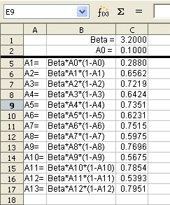
Splitting
the screen
Another way to change the view is by splitting the window, also known as splitting the screen. The screen can be split horizontally, vertically, or both. You can therefore have up to four portions of the spreadsheet in view at any one time.
Why would you want to do this? An example would be a large spreadsheet in which one of the cells has a number in it that is used by three formulas in other cells. Using the split-screen technique, you can position the cell containing the number in one section and each of the cells with formulas in the other sections. Then you can change the number in the cell and watch how it affects each of the formulas.
Splitting the screen horizontally
To split the screen horizontally:
Move the mouse pointer into the vertical scroll bar, on the right-hand side of the screen, and place it over the small button at the top with the black triangle.
Immediately above this button, you will see a thick black line (Figure 28). Move the mouse pointer over this line, and it turns into a line with two arrows (Figure 29).
Hold down the left mouse button. A gray line appears, running across the page. Drag the mouse downwards and this line follows.
Release the mouse button and the screen splits into two views, each with its own vertical scroll bar. You can scroll the upper and lower parts independently.
Notice in Figure 27, the Beta and the A0 values are in the upper part of the window and other calculations are in the lower part. Thus, you can make changes to the Beta and A0 values and watch their effects on the calculations in the lower half of the window.
|
Tip |
You can also split the screen using a menu command. Click in a cell immediately below and to the right of where you wish the screen to be split, and choose Window → Split. |
Splitting the screen vertically
To split the screen vertically:
Move the mouse pointer into the horizontal scroll bar at the bottom of the screen and place it over the small button on the right with the black triangle.
Immediately to the right of this button is a thick black line (Figure 30). Move the mouse pointer over this line and it turns into a line with two arrows.
Hold down the left mouse button, and a gray line appears, running up the page. Drag the mouse to the left and this line follows.
Release the mouse button, and the screen is split into two views, each with its own horizontal scroll bar. You can scroll the left and right parts of the window independently.
Removing split views
To remove a split view, do any of the following:
Double-click on each split line.
Click on and drag the split lines back to their places at the ends of the scroll bars.
Choose Window → Split to remove all split lines at the same time.
In addition to the cell reference boxes (labeled Column and Row), the Navigator provides several other ways to move quickly through a spreadsheet and find specific items.
To
open the Navigator, click its icon
![]() on the Standard toolbar, or
press F5,
or choose View
→ Navigator on
the Menu bar, or double-click on the Sheet Sequence Number
on the Standard toolbar, or
press F5,
or choose View
→ Navigator on
the Menu bar, or double-click on the Sheet Sequence Number
![]() in the Status Bar. You can dock the Navigator to either side
of the main Calc window or leave it floating. (To dock or float the
Navigator, hold down the Control
key and double-click in an empty area near the icons at the top.)
in the Status Bar. You can dock the Navigator to either side
of the main Calc window or leave it floating. (To dock or float the
Navigator, hold down the Control
key and double-click in an empty area near the icons at the top.)
The Navigator displays lists of all the objects in a spreadsheet document, grouped into categories. If an indicator (plus sign or arrow) appears next to a category, at least one object of this kind exists. To open a category and see the list of items, click on the indicator.
To
hide the list of categories and show only the icons at the top, click
the Contents
icon
![]() .
Click this icon again to show the list.
.
Click this icon again to show the list.
Table 2 summarizes the functions of the icons at the top of the Navigator.
Table 2: Function of icons in the Navigator
|
Icon |
Action |
|
|
Data Range. Specifies the current data range denoted by the position of the cell cursor. |
|
|
Start/End. Moves to the cell at the beginning or end of the current data range, which you can highlight using the Data Range button. |
|
|
Contents. Shows or hides the list of categories. |
|
|
Toggle. Switches between showing all categories and showing only the selected category. |
|
|
Displays all available scenarios. Double-click a name to apply that scenario. See Chapter 9, Data Analysis, for more information. |
|
|
Drag Mode. Choose hyperlink, link, or copy. See “Choosing a drag mode” for details. |
Moving quickly through a document
The Navigator provides several convenient ways to move around a document and find items in it:
To jump to a specific cell in the current sheet, type its cell reference in the Column and Row boxes at the top of the Navigator and press the Enter key; for example, in Figure 31 the cell reference is A7.
When a category is showing the list of objects in it, double-click on an object to jump directly to that object’s location in the document.
To see the content in only one category, highlight that category and click the Toggle icon. Click the icon again to display all the categories.
Use the Start and End icons to jump to the first or last cell in the selected data range.
|
Tip |
Ranges, scenarios, pictures, and other objects are much easier to find if you have given them informative names when creating them, instead of keeping Calc’s default Graphics 1, Graphics 2, Object 1, and so on, which may not correspond to the position of the object in the document. |
Sets the drag and drop options for inserting items into a document using the Navigator.
Insert as Hyperlink
Creates a hyperlink when you drag and drop an item into the current document.
Insert as Link
Inserts the selected item as a link where you drag and drop an object into the current document.
Insert as Copy
Inserts a copy of the selected item where you drag and drop in the current document. You cannot drag and drop copies of graphics, OLE objects, or indexes.
To open the Properties dialog for a document, choose File → Properties.
The Properties dialog has six tabs. The information on the General page and the Statistics page is generated by the program. Other information (the name of the person on the Created and Modified lines of the General page) is derived from the User Data page in Tools → Options.
The Internet page is relevant only to HTML documents. The file sharing options on the Security page are discussed elsewhere in this book.
Use the Description and Custom Properties pages to hold:
Metadata to assist in classifying, sorting, storing, and retrieving documents. Some of this metadata is exported to the closest equivalent in HTML and PDF; some fields have no equivalent and are not exported.
Information that changes. You can store data for use in fields in your document; for example, the title of the document, contact information for a project participant, or the name of a product might change during the course of a project.
This dialog can be used in a template, where the field names can serve as reminders to users of information they need to include.
You can return to this dialog at any time and change the information you entered. When you do so, all of the references to that information will change wherever they appear in the document. For example, on the Description page (Figure 32) you might need to change the contents of the Title field from the draft title to the final title.
Use the Custom Properties page (Figure 33) to store information that does not fit into the fields supplied on the other pages of this dialog box.
When the Custom Properties page is first opened in a new document, it may be blank. However, if the new document is based on a template, this page may contain fields.
Click Add to insert a row of boxes into which you can enter your custom properties.
The Name box includes a drop-down list of typical choices; scroll down to see all the choices. If none of the choices meet your needs, you can type a new name into the box.
In the Type column, you can choose from text, date+time, date, number, duration, or yes/no for each field. You cannot create new types.
In the Value column, type or select what you want to appear in the document where this field is used. Choices may be limited to specific data types depending on the selection in the Type column; for example, if the Type selection is Date, the Value for that property is limited to a date.
To remove a custom property, click the button at the end of the row.
|
Tip |
To change the format of the Date value, go to Tools → Options → Languages and change the Locale setting. Be careful! This change affects all open documents, not just the current one. |