Calc Guide

Chapter 10
Linking Calc Data

Sharing data in and out of Calc

Why use multiple sheets?

Chapter 1 introduced the concept of multiple sheets in a spreadsheet. Multiple sheets help keep information organized; once you link those sheets together, you unleash the full power of Calc. Consider this case.

Setting up multiple sheets

Chapter 1 gives a detailed explanation of how to set up multiple sheets in a spreadsheet. Here is a quick review.

Identifying sheets

When you open a new spreadsheet it has, by default, three sheets named Sheet1, Sheet2, and Sheet3. Sheets in Calc are managed using tabs at the bottom of the spreadsheet.

Inserting new sheets

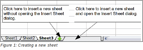
There are several ways to insert a new sheet. The fastest method is to click on the Add Sheet button . This inserts one new sheet at that point, without opening the Insert Sheet dialog.

Use one of the other methods to insert more than one sheet, to rename the sheet at the same time, or to insert the sheet somewhere else in the sequence. The first step for these methods is to select the sheet that the new sheet will be inserted next to. Then do any of the following:

• Select Insert → Sheet from the menu bar, or

• Right-click on the tab and select Insert Sheet, or

• Click in an empty space at the end of the line of sheet tabs.

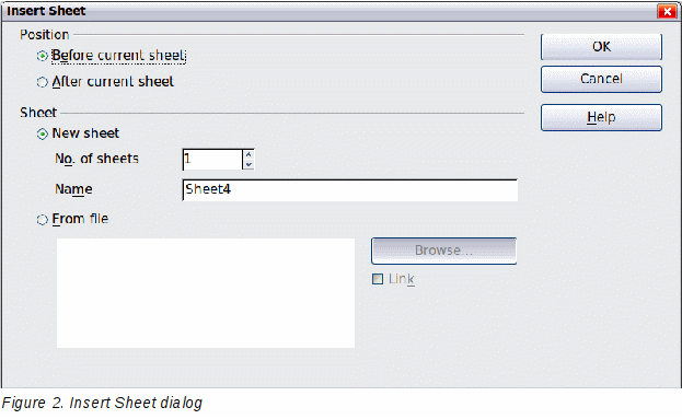
Each method opens the Insert Sheet dialog. Here you can choose to put the new sheet before or after the selected sheet and how many sheets to insert.

We need 6 sheets, one for each of the 5 accounts and one as a summary sheet, so we will add 3 more. We also want to name each of these sheets for the account they represent: Summary, Checking Account, Savings Account, Credit Card 1, Credit Card 2, and Car Loan.

We have two choices: insert 3 new sheets and rename all 6 sheets afterwards; or rename the existing sheets, then insert the 3 new sheets one at a time, renaming each new sheet during the insert step.

To insert sheets and rename afterwards:

1. In the Insert Sheet dialog, choose the position for the new sheets (in this example, we use After current sheet).

2. Choose New sheet and 3 as the No. of sheets. (Three sheets are already provided by default.) Because you are inserting more than one sheet, the Name box is not available.

3. Click OK to insert the sheets.

4. For the next steps, go to “Renaming sheets” on page 6.

To insert sheets and name them at the same time:

1. Rename the existing sheets Summary, Checking Account, and Savings Account, as described in “Renaming sheets” on page 6.

2. In the Insert Sheet dialog, choose the position for the first new sheet.

3. Choose New sheet and 1 as the No. of sheets. The Name box is now available.

4. In the Name box, type a name for this new sheet, for example Credit Card 1.

5. Click OK to insert the sheet.

6. Repeat steps 1–4 for each new sheet, giving them the names Credit Card 2 and Car Loan.

Inserting sheets from a different spreadsheet

On the Insert Sheet dialog, you can also add a sheet from a different spreadsheet file (for example, another Calc or Excel spreadsheet), by choosing the From file option. Click Browse and select the file; a list of the available sheets appears in the box. Select the sheet to import. If, after you select the file, no sheets appear you probably selected an invalid file type (not a spreadsheet, for example).

If you prefer, select the Link option to insert the external sheet as a link instead as a copy. This is one of several ways to include “live” data from another spreadsheet. (See also “Linking to external data” on page 13.) The links can be updated manually to show the current contents of the external file; or, depending on the options you have selected in Tools → Options → LibreOffice Calc → General → Updating, whenever the file is opened.

Renaming sheets

Sheets can be renamed at any time. To give a sheet a more meaningful name:

• Enter the name in the name box when you create the sheet, or

• Double click on the sheet tab, or

• Right-click on a sheet tab, select Rename Sheet from the context menu and replace the existing name.

Your sheet tab area should now look like this.

Now we will set up the account ledgers. This is just a simple summary that includes the previous balance plus the amount of the current transaction. For withdrawals, we enter the current transaction as a negative number so the balance gets smaller. A basic ledger is shown in Figure 4.

This ledger is set up in the sheet named Checking Account. The total balance is added up in cell F3. You can see the equation for it in the formula bar. It is the summary of the opening balance, cell C3, and all of the subsequent transactions.

Referencing other sheets

On the Summary sheet we display the balance from each of the other sheets. If you copy the example in Figure 4 onto each account, the current balances will be in cell F3 of each sheet.

There are two ways to reference cells in other sheets: by entering the formula directly using the keyboard or by using the mouse. We will look at the mouse method first.

Creating the reference with the mouse

On the Summary sheet, set up a place for all five account balances, so we know where to put the cell reference. Figure 5 shows a summary sheet with a blank Balance column. We want to place the reference for the checking account balance in cell B3.

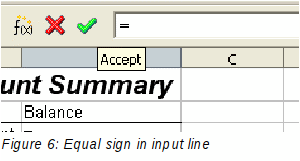
To make the cell reference in cell B3, select the cell and follow these steps:

1. Click on the = icon next to the input line. The icons change and an equals sign appears in the input line as in Figure 6.

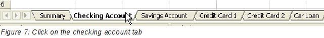
2. Now, click on the sheet tab for the sheet containing the cell to be referenced. In this case, that is the Checking Account sheet as shown in Figure 7.

3. Click on cell F3 (where the balance is) in the Checking Account sheet. The phrase ‘Checking Account’.F3 should appear in the input line as in Figure 8.

4. Click the green checkmark in the input line to finish.

5. The Summary sheet should now look like Figure 9.

Creating the reference with the keyboard

From Figure 9, you can deduce how the cell reference is constructed. The reference has two parts: the sheet name (‘Checking Account’) and the cell reference (F3). Notice that they are separated by a period.

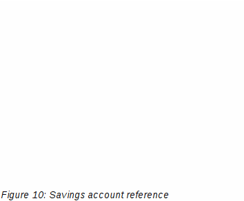
So, you can fill in the Savings Account cell reference by just typing it in. Assuming that the balance is in the same cell (F3) in the Savings Account sheet, the cell reference should be =’Savings Account’.F3 (see Figure 10).

Referencing other documents

John decides to keep his family account information in a different spreadsheet file from his own summary. Fortunately Calc can link different files together. The process is the same as described for different sheets in a single spreadsheet, but we add one more step to indicate which file the sheet is in.

Creating the reference with the mouse

To create the reference with the mouse, both spreadsheets need to be open. Select the cell in which the formula is going to be entered.

1. Click the = icon next to the input line.

2. Switch to the other spreadsheet (the process to do this will vary depending on which operating system you are using).

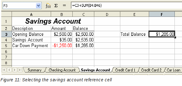
3. Select the sheet (Savings Account) and then the reference cell (F3). See Figure 11.

4. Switch back to the original spreadsheet.

5. Click on the green check mark on the input line.

Your spreadsheet should now resemble Figure 12.

You will get a good feel for the format of the reference if you look closely at the input line. Based on this line you can create the reference using the keyboard.

Creating the reference with the keyboard

Typing the reference is simple once you know the format the reference takes. The reference has three parts to it:

• Path and file name

• Sheet name

• Cell

Looking at Figure 12 you can see the the general format for the reference is

=’file:///Path & File Name’#$SheetName.CellName

Hyperlinks and URLs

Hyperlinks can be used in Calc to jump to a different location from within a spreadsheet and can lead to other parts of the current file, to different files or even to web sites.

Relative and absolute hyperlinks

Hyperlinks can be stored within your file as either relative or absolute.

A relative hyperlink says, Here is how to get there starting from where you are now (meaning from the folder in which your current document is saved) while an absolute hyperlink says, Here is how to get there no matter where you start from.

An absolute link will stop working only if the target is moved. A relative link will stop working only if the start and target locations change relative to each other. For instance, if you have two spreadsheets in the same folder linked to each other and you move the entire folder to a new location, a relative hyperlink will not break.

To change the way that LibreOffice stores the hyperlinks in your file, select Tools → Options → Load/Save → General and choose if you want URLs saved relatively when referencing the File System, or the Internet, or both.

Calc will always display an absolute hyperlink. Don’t be alarmed when it does this even when you have saved a relative hyperlink—this ‘absolute’ target address will be updated if you move the file.

Creating hyperlinks

When you type text that can be used as a hyperlink (such as a website address or URL), Calc formats it automatically, creating the hyperlink and applying to the text a color and background shading. If this does not happen, you can enable this feature using Tools → AutoCorrect Options → Options and selecting URL Recognition.

You can also insert and modify links using the Hyperlink dialog. To display the dialog, click the Hyperlink icon on the Standard toolbar or choose Insert → Hyperlink from the menu bar. To turn existing text into a link, highlight it before opening the dialog.

On the left side, select one of the four categories of hyperlinks:

• Internet: the hyperlink points to a web address, normally starting with http://

• Mail & News: the hyperlink opens an email message that is pre-addressed to a particular recipient.

• Document: the hyperlink points to a place in either the current document or another existing document.

• New document: the hyperlink creates a new document.

The top right part of the dialog changes according to the choice made for the hyperlink category from the left panel. A full description of all the choices, and their interactions, is beyond the scope of this chapter. Here is a summary of the most common choices used in spreadsheets.

For an Internet hyperlink, choose the type of hyperlink (Web, FTP, or Telnet), and enter the required web address (URL).

For a Mail and News hyperlink, specify whether it is a mail or news link, the receiver address and for email, also the subject.

For a Document hyperlink, specify the document path (the Open File button opens a file browser); leave this blank if you want to link to a target in the same spreadsheet. Optionally specify the target in the document (for example a specific sheet). Click on the Target in document icon to open the Navigator where you can select the target, or if you know the name of the target, you can type it into the box.

For a New Document hyperlink, specify whether to edit the newly created document immediately (Edit now) or just create it (Edit later), and enter the file name and the type of document to create (text, spreadsheet, etc.). The Select path button opens a directory picker dialog.

The Further settings section in the bottom right of the dialog is common to all the hyperlink categories, although some choices are more relevant to some types of links.

• Set the value of Frame to determine how the hyperlink will open. This applies to documents that open in a Web browser.

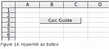
• Form specifies if the link is to be presented as text or as a button. Figure 14 shows a link formatted as a button.

• Text specifies the text that will be visible to the user. If you do not enter anything here, Calc will use the full URL or path as the link text. Note that if the link is relative and you move the file, this text will not change, though the target will.

• Name is applicable to HTML documents. It specifies text that will be added as a NAME attribute in the HTML code behind the hyperlink.

• Events button: this button will be activated to allow Calc to react to events for which the user has written some code (macro). This function is not covered in this chapter.

Editing hyperlinks

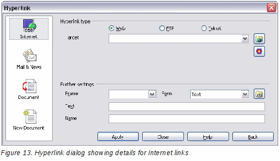
To edit an existing link, place the cursor anywhere in the link and click the Hyperlink icon on the Standard toolbar or select Edit → Hyperlink from the menu bar. The Hyperlink dialog (Figure 13) opens. If the Hyperlink is in button form, the spreadsheet must have Design Mode on in order to edit the Hyperlink. Make your changes and click Apply. If you need to edit several hyperlinks, you can leave the Hyperlink dialog open until you have edited all of them. Be sure to click Apply after each one. When you are finished, click Close.

Removing hyperlinks

You can remove the clickable link from hyperlink text—leaving just the text—by right-clicking on the link and selecting Default Formatting. This option is also available from the Format menu. You may then need to re-apply some formatting in order for it to match the rest of your document.

To erase the link text or button from the document completely, select it and press the Backspace or Delete key.

Linking to external data

You can insert tables from HTML documents, and data located within named ranges from a LibreOffice Calc or Microsoft Excel spreadsheet, into a Calc spreadsheet. (To use other data sources, including database files in LibreOffice Base, see “Linking to registered data sources” on page 18.)

You can do this in two ways: using the External Data dialog or using the Navigator. If your file has named ranges or named tables, and you know the name of the range or table you want to link to, using the External Data dialog method is quick and easy. However, if the file has several tables, and you want to pick only one of them, you may not be able to easily determine which is which; in that case, the Navigator method may be easier.

Using the External Data dialog

1. Open the Calc document where the external data is to be inserted. This is the target document.

2. Select the cell where the upper left-hand cell of the external data is to be inserted.

3. Choose Insert → Link to External Data.

4. On the External Data dialog, type the URL of the source document or click the [...] button to open a file selection dialog. Press Enter to get Calc to load the list of available tables.

5. In the Available tables/range list, select the named ranges or tables you want to insert. You can also specify that the ranges or tables are updated every (number of) seconds.

6. Click OK to close the dialog and insert the linked data.

Using the Navigator

1. Open the Calc spreadsheet in which the external data is to be inserted (target document).

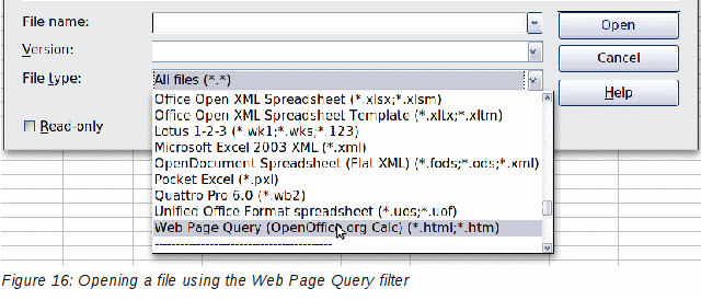
2. Open the document from which the external data is to be taken (source document). If the source document is a Web page, choose Web Page Query (LibreOffice Calc) as the file type.

3. In the target document, press F5 to open the Navigator.

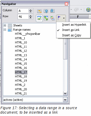
4. At the bottom of the Navigator, select the source document. (In Figure 17, the source is named actives.)

The Navigator now shows the range names or the tables contained in the source document (the example contains range names; other documents have a list of tables). Click on the + next to Range names to display the list.

5. In the Navigator, select the Insert as Link drag mode, as shown in Figure 17.

6. Select the required range or table and drag it from the Navigator into the target document, to the cell where you want the upper left-hand cell of the data range to be.

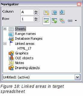
7. In the target document, check the Navigator. Instead of a + by Range names, it shows a + by Linked areas. Click the + to see the same range name (see Figure 18).

How to find the required data range or table

The examples above show that the import filter gave names to the data ranges (tables) in the sample web page starting from HTML_1. It also created two additional range names (not visible in the illustration):

HTML_all – designates the entire document

HTML_tables – designates all HTML tables in the document

If the data tables in the source HTML document have been given names (using the ID attribute on the TABLE tag), or the external spreadsheet includes named ranges, those names appear in the list along with the ranges Calc has sequentially numbered.

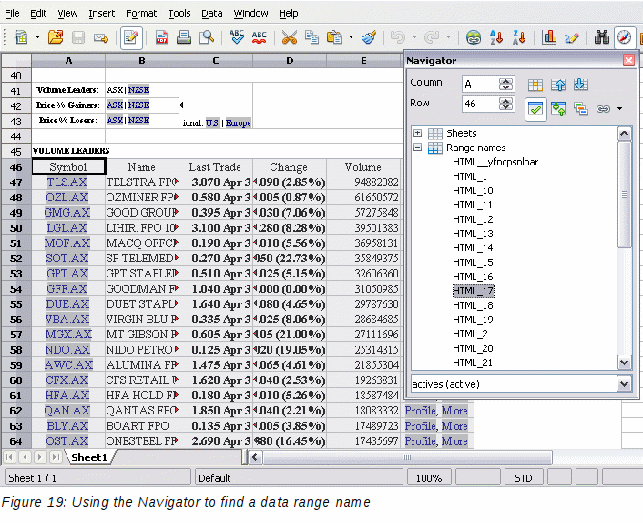
If the data range or table you want is not named, how can you tell which one to select?

Go to the source document, which you opened in Calc. In the Navigator, double-click on a range name: that range is highlighted on the sheet (see Figure 19).

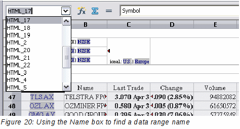
If the Formula Bar is visible, the range name is also displayed in the Name box at the left-hand end (see Figure 20).

Linking to registered data sources

You can access a variety of databases and other data sources and link them into Calc documents.

First you need to register the data source with LibreOffice. (To register means to tell LibreOffice what type of data source it is and where the file is located.) The way to do this depends on whether or not the data source is a database in *.odb format.

To register a data source that is in *.odb format:

1. Choose Tools → Options → LibreOffice Base → Databases.

2. Click the New button (below the list of registered databases) to open the Create Database Link dialog (Figure 21).

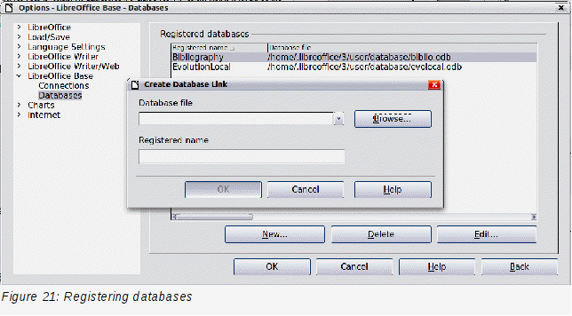
3. Enter the location of the database file, or click Browse to open a file browser and select the database file.

4. Type a name to use as the registered name for the database and click OK. The database is added to the list of registered databases. The OK button is enabled only when both fields are filled in.

To register a data source that is not in *.odb format:

1. Choose File → New → Database to open the Database Wizard.

2. Select Connect to an existing database. The choices for database type depend on your operating system. For example, Microsoft Access and other Microsoft products are not among the choices if you are using Linux. In our example, we chose dBASE.

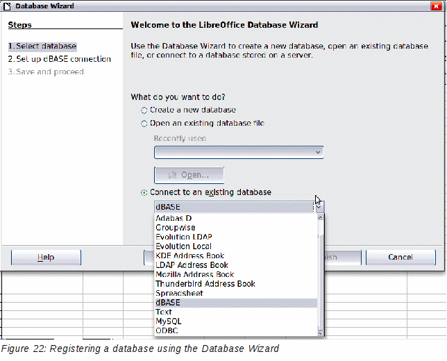
3. Click Next. Type the path to the database file or click Browse and use the Open dialog to navigate to and select the database file before clicking Open.

4. Click Next. Select Yes, register the database for me, but clear the checkbox marked Open the database for editing.

5. Click Finish. Name and save the database in the location of your choice. Note: changes made to the *.odb do not affect the original dBASE file.

Once a data source has been registered, it can be used by any LibreOffice component (for example Calc).

Viewing data sources

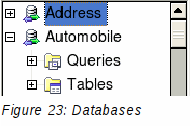
Open a document in Calc. To view the data sources available, press F4 or select View → Data Sources from the menu bar. The Data Source View pane opens above the spreadsheet. A list of registered databases is in the Data Explorer area on the left. (The built-in Bibliography database is included in the list.)

To view each database, click on the + to the left of the name of the database. (This has been done for the Automobile database in Figure 23.) Click on the + next to Tables to view the individual tables.

Now click on a table to see all the records held in it. The data records are displayed on the right side of the Data Source View pane. To see more columns, you can click the Explorer On/Off button to hide the Data Explorer area.

At the top of the Data Source View pane, below the Calc toolbars, is the Table Data bar. This toolbar includes buttons for saving records, editing data, finding records, sorting, filtering, and other functions. For more details about this toolbar, see the Help for data source browser.

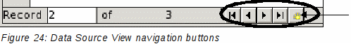
Below the records is the Form Navigation bar, which shows which record is selected and the total number of records. To the right are five tiny buttons; the first four move backwards or forwards through the records, or to the beginning or end.

Editing data sources

Some data sources (such as spreadsheets) cannot be edited in the data source view.

In editable data sources, records can be edited, added, or deleted. If you cannot save your edits, you need to open the database in Base and edit it there; see “Launching Base to work on data sources”. You can also hide columns and make other changes to the display.

Launching Base to work on data sources

You can launch LibreOffice Base at any time from the Data Source View pane. Right-click on a database or the Tables or Queries icons and select Edit Database File. Once in Base, you can edit, add, and delete tables, queries, forms, and reports.

For more about using Base, see Chapter 8, Getting Started with Base, in the Getting Started guide.

Using data sources in Calc spreadsheets

Data from the tables in the data source pane can be placed into Calc documents in a variety of ways.

You can select a cell or an entire row in the data source pane and drag and drop the data into the spreadsheet. The data is inserted at the place where you release the mouse button.

An alternative method uses the Data to Text icon and will include the column headings above the data you insert:

1. Click the cell of the spreadsheet which you want to be the top left of your data including the column names.

2. Press F4 to open the database source window and select the table containing the data you want to use.

3. Select the rows of data you want to add to the spreadsheet:

• Click the gray box to the left of the row you want to select if only selecting one row. That row is highlighted.

• To select multiple adjacent rows, hold down the Shift key while clicking the gray box of the rows you need.

• To select multiple separate rows, hold down the Control key while selecting the rows. The selected rows are highlighted.

• To select all the rows, click the gray box in the upper left corner. All rows are highlighted.

4. Click the Data to text icon to insert the data into the spreadsheet cells.

You can also drag the data source column headings (field names) onto your spreadsheet to create a form for viewing and editing individual records one at a time. Follow these steps:

1. Click the gray box at the top of the column (containing the field name you wish to use) to highlight it.

2. Drag and drop the gray box to where you want the record to appear in the spreadsheet.

3. Repeat until you have moved all of the fields you need to where you want them.

4. Close the Data Source window: press F4.

5. Save the spreadsheet and click the Edit File button on the Standard toolbar, to make the spreadsheet read-only. All of the fields will show the value for the data of the first record you selected.

6. Add the Form Navigation toolbar: View → Toolbars → Form Navigation. By default, this toolbar opens at the bottom of the Calc window, just above the status bar.

7. Click the arrows on the Form Navigation toolbar to view the different records of the table. The number in the Record box changes as you move through the records. The data in the fields changes to correspond to the data for that particular record number. You can also search for a specific record, sort and filter records, and do other tasks using this toolbar.

Embedding spreadsheets

Spreadsheets can be embedded in other LibreOffice files. This is often used in Writer or Impress documents so that Calc data can be used in a text document. You can embed the spreadsheet as either an OLE or DDE object. The difference between a DDE object and a Linked OLE object is that a Linked OLE object can be edited from the document in which it is added as a link, but a DDE object cannot.

For example, if a Calc spreadsheet is pasted into a Writer document as a DDE object, then the spreadsheet cannot be edited in the Writer document. But if the original Calc spreadsheet is updated, the changes are automatically made in the Writer document. If the spreadsheet is inserted as a Linked OLE object into the Writer document, then the spreadsheet can be edited in the Writer as well as in the Calc document and both documents are in sync with each other.

Object Linking and Embedding (OLE)

The major benefit of an OLE (Object Linking and Embedding) object is that it is quick and easy to edit the contents just by double-clicking on it. You can also insert a link to the object that will appear as an icon rather than an area showing the contents itself.

OLE objects can be linked to a target document or be embedded in the target document. Linking inserts information which will be updated with any subsequent changes to the original file, while embedding inserts a static copy of the data. If you want to edit the embedded spreadsheet, double-click on the object.

To embed a spreadsheet as an OLE object in a presentation:

1. Place the cursor in the document and location you want the OLE object to be.

2. Select Insert → Object → OLE Object. The dialog below opens.

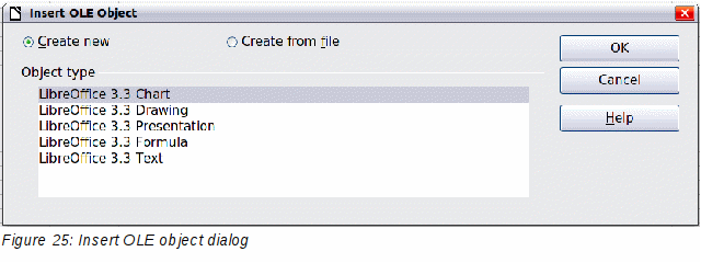
3. You can either create a new OLE object or create from a file.

To create a new object:

1. Select Create new and select the object type among the available options.

2. Click OK. An empty container is placed in the slide.

3. Double-click on the OLE object to enter the edit mode of the object. The application devoted to handling that type of file will open the object.

To insert an existing object:

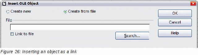
1. To create from a file, select Create from file. The dialog changes to look like Figure 26.

2. To insert the object as a link, select the Link to file option. Otherwise, the object will be embedded.

3. Click Search, select the required file in the Open dialog, then click Open. A section of the inserted file is shown in the document.

Other OLE objects

Under Windows, the Insert OLE Object dialog box has an extra entry, Further objects.

1. Double-click on the entry Further objects to open the dialog shown below.

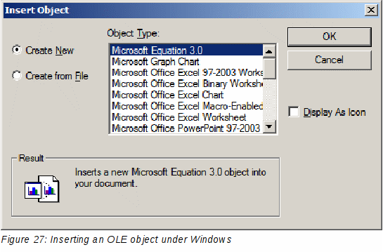
2. Select Create New to insert a new object of the type selected in the Object Type list, or select Create from File to create a new object from a file.

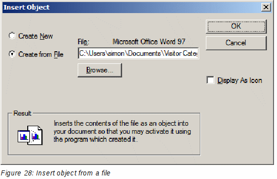
3. If you choose Create from File, the dialog shown below opens. Click Browse and choose the file to insert. The inserted file object is editable by the Windows program that created it.

If instead of inserting an object, you want to insert a link to an object, select the Display As Icon option.

Non-linked OLE object

If the OLE object is not linked, it can be edited in the new document. For instance, if you insert a spreadsheet into a Writer document, you can essentially treat it as a Writer table (with a little more power). To edit it, double-click on it.

Linked OLE object

When the spreadsheet OLE object is linked, if you change it in Writer it will change in Calc; if you change it in Calc, it will change in Writer. This can be a very powerful tool if you create reports in Writer using Calc data, and want to make a quick change without opening Calc.

Dynamic Data Exchange (DDE)

DDE is an acronym for Dynamic Data Exchange, a mechanism whereby selected data in document A can be pasted into document B as a linked, ‘live’ copy of the original. It would be used, for example, in a report written in Writer containing time varying data, such as sales results sourced from a Calc spreadsheet. The DDE link ensures that, as the source spreadsheet is updated so is the report, thus reducing the scope for error and reducing the work involved in keeping the Writer document up to date.

DDE is a predecessor of OLE. With DDE, objects are linked through file reference, but not embedded. You can create DDE links either within Calc cells in a Calc sheet, or in Calc cells in another LibreOffice doc such as in Writer.

DDE link in Calc

Creating a DDE link in Calc is similar to creating a cell reference. The process is a little different, but the result is the same.

1. In Calc, select the cells that you want to make the DDE link to.

2. Copy them: Edit → Copy or Ctrl+C.

3. Go to the place in the spreadsheet where you want the link to be.

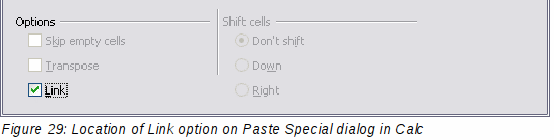
4. Select Edit → Paste Special.

5. When the Paste Special dialog opens, select the Link option on the bottom left of the dialog (Figure 29). Click OK.

The cells now reference the copied data, and the formula bar shows a reference beginning with {=DDE.

If you now edit the original cells, the linked cells will update.

DDE link in Writer

The process for creating a DDE link from Calc to Writer is similar to creating a link within Calc.

1. In Calc, select the cells to make the DDE link to. Copy them.

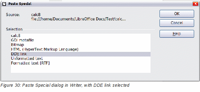
2. Go to the place in your Writer document where you want the DDE link. Select Edit → Paste Special.

3. Select DDE Link (Figure 30). Click OK.

Now the link has been created in Writer. When the Calc spreadsheet is updated, the table in Writer is automatically updated.