Calc Guide

Chapter 2
Entering, Editing, and Formatting Data

Introduction

You can enter data into Calc in several ways: using the keyboard, the mouse (dragging and dropping), the Fill tool, and selection lists. Calc also provides the ability to enter information into multiple sheets of the same document at the same time.

After entering data, you can format and display it in various ways.

Entering data using the keyboard

Most data entry in Calc can be accomplished using the keyboard.

Entering numbers

Click in the cell and type in the number using the number keys on either the main keyboard or the numeric keypad.

To enter a negative number, either type a minus (–) sign in front of it or enclose it in parentheses (brackets), like this: (1234).

By default, numbers are right-aligned and negative numbers have a leading minus symbol.

Entering text

Click in the cell and type the text. Text is left-aligned by default.

Entering numbers as text

If a number is entered in the format 01481, Calc will drop the leading 0. (Exception: see Tip below.) To preserve the leading zero, for example for telephone area codes, type an apostrophe before the number, like this: '01481.

The data is now treated as text and displayed exactly as entered. Typically, formulas will treat the entry as a zero and functions will ignore it.

Entering dates and times

Select the cell and type the date or time. You can separate the date elements with a slash (/) or a hyphen (–) or use text such as 10 Oct 03. Calc recognizes a variety of date formats. You can separate time elements with colons such as 10:43:45.

Entering special characters

A “special” character is one not found on a standard English keyboard. For example, © ¾ æ ç ñ ö ø ¢ are all special characters. To insert a special character:

1. Place the cursor in your document where you want the character to appear.

2. Click Insert → Special Character to open the Special Characters dialog (Figure 1).

3. Select the characters (from any font or mixture of fonts) you wish to insert, in order; then click OK. The selected characters are shown in the bottom left of the dialog. As you select each character, it is shown alone at the bottom right, along with the numerical code for that character.

Inserting dashes

To enter en and em dashes, you can use the Replace dashes option under Tools → AutoCorrect Options → Options tab. This option replaces two hyphens, under certain conditions, with the corresponding dash.

In the following table, the A and B represent text consisting of letters A to z or digits 0 to 9.

Deactivating automatic changes

Calc automatically applies many changes during data input, unless you deactivate those changes. You can also immediately undo any automatic changes with Ctrl+Z.

AutoCorrect changes

Automatic correction of typing errors, replacement of straight quotation marks by curly (custom) quotes, and starting cell content with an uppercase (capital) letter are controlled by Tools → AutoCorrect Options. Go to the Options or Replace tabs to deactivate any of the features that you do not want. On the Replace tab, you can also delete unwanted word pairs and add new ones as required.

AutoInput

When you are typing in a cell, Calc automatically suggests matching input found in the same column. To turn the AutoInput on and off, set or remove the check mark in front of Tools → Cell Contents → AutoInput.

Automatic date conversion

Calc automatically converts certain entries to dates. To ensure that an entry that looks like a date is interpreted as text, type an apostrophe at the beginning of the entry. The apostrophe is not displayed in the cell.

Speeding up data entry

Entering data into a spreadsheet can be very labor-intensive, but Calc provides several tools for removing some of the drudgery from input.

The most basic ability is to drop and drag the contents of one cell to another with a mouse. Many people also find AutoInput helpful. Calc also includes several other tools for automating input, especially of repetitive material. They include the Fill tool, selection lists, and the ability to input information into multiple sheets of the same document.

Using the Fill tool on cells

At its simplest, the Fill tool is a way to duplicate existing content. Start by selecting the cell to copy, then drag the mouse in any direction (or hold down the Shift key and click in the last cell you want to fill), and then choose Edit → Fill and the direction in which you want to copy: Up, Down, Left or Right.

Using a fill series

A more complex use of the Fill tool is to use a fill series. The default lists are for the full and abbreviated days of the week and the months of the year, but you can create your own lists as well.

To add a fill series to a spreadsheet, select the cells to fill, choose Edit → Fill → Series. In the Fill Series dialog, select AutoFill as the Series type, and enter as the Start value an item from any defined series. The selected cells then fill in the other items on the list sequentially, repeating from the top of the list when they reach the end of the list.

You can also use Edit → Fill → Series to create a one-time fill series for numbers by entering the start and end values and the increment. For example, if you entered start and end values of 1 and 7 with an increment of 2, you would get the sequence of 1, 3, 5, 7.

In all these cases, the Fill tool creates only a momentary connection between the cells. Once they are filled, the cells have no further connection with one another.

Defining a fill series

To define your own fill series, go to Tools → Options → LibreOffice Calc → Sort Lists. This dialog shows the previously-defined series in the Lists box on the left, and the contents of the highlighted list in the Entries box.

Click New. The Entries box is cleared. Type the series for the new list in the Entries box (one entry per line), and then click Add.

Using selection lists

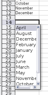
Selection lists are available only for text, and are limited to using only text that has already been entered in the same column.

To use a selection list, select a blank cell and press Ctrl+D. A drop-down list appears on any cell in the same column that either has at least one text character or whose format is defined as text. Click on the entry you require.

Sharing content between sheets

You might want to enter the same information in the same cell on multiple sheets, for example to set up standard listings for a group of individuals or organizations. Instead of entering the list on each sheet individually, you can enter it in all the sheets at once. To do this, select all the sheets (Edit → Sheet → Select), then enter the information in the current one.

Validating cell contents

When creating spreadsheets for other people to use, you may want to make sure they enter data that is valid or appropriate for the cell. You can also use validation in your own work as a guide to entering data that is either complex or rarely used.

Fill series and selection lists can handle some types of data, but they are limited to predefined information. To validate new data entered by a user, select a cell and use Data → Validity to define the type of contents that can be entered in that cell. For example, a cell might require a date or a whole number, with no alphabetic characters or decimal points; or a cell may not be left empty.

Depending on how validation is set up, the tool can also define the range of values that can be entered and provide help messages that explain the content rules you have set up for the cell and what users should do when they enter invalid content. You can also set the cell to refuse invalid content, accept it with a warning, or—if you are especially well-organized—start a macro when an error is entered.

Validation is most useful for cells containing functions. If cells are set to accept invalid content with a warning, rather than refusing it, you can use Tools → Detective → Mark Invalid Data to find the cells with invalid data. The Detective function marks any cells containing invalid data with a circle.

Note that a validity rule is considered part of a cell’s format. If you select Format or Delete All from the Delete Contents window, then it is removed. (Repeating the Detective’s Mark Invalid Data command removes the invalid data circle, because the data is no longer invalid.) If you want to copy a validity rule with the rest of the cell, use Edit → Paste Special → Paste Formats or Paste All.

Figure 7 shows the choices for a typical validity test. Note the Allow blank cells option under the Allow list.

The validity test options vary with the type of data selected from the Allow list. For example, Figure 8 shows the choices when a cell must contain a cell range.

To provide input help for a cell, use the Input Help page of the Validity dialog (Figure 9). To show an error message when an invalid value is entered, use the Error Alert page (Figure 10). Be sure to write something helpful, explaining what a valid entry should contain—not just “Invalid data—try again” or something similar.

Editing data

Editing data is done is in much the same way as entering it. The first step is to select the cell containing the data to be edited.

Removing data from a cell

Data can be removed (deleted) from a cell in several ways.

Removing data only

The data alone can be removed from a cell without removing any of the formatting of the cell. Click in the cell to select it, and then press the Backspace key.

Removing data and formatting

The data and the formatting can be removed from a cell at the same time. Press the Delete key (or right-click and choose Delete Contents, or use Edit → Delete Contents) to open the Delete Contents dialog (Figure 11). From this dialog, different aspects of the cell can be deleted. To delete everything in a cell (contents and format), check Delete all.

Replacing all the data in a cell

To remove data and insert new data, simply type over the old data. The new data will retain the original formatting.

Changing part of the data in a cell

Sometimes it is necessary to change the contents of a cell without removing all of the contents, for example when the phrase “See Dick run” is in a cell and it needs to be changed to “See Dick run fast.” It is often useful to do this without deleting the old cell contents first.

The process is the similar to the one described above, but you need to place the cursor inside the cell. You can do this in two ways.

Using the keyboard

After selecting the appropriate cell, press the F2 key and the cursor is placed at the end of the cell. Then use the keyboard arrow keys to move the cursor through the text in the cell.

Using the mouse

Using the mouse, either double-click on the appropriate cell (to select it and place the cursor in it for editing), or single-click to select the cell and then move the mouse pointer up to the input line and click into it to place the cursor for editing.

Formatting data

The data in Calc can be formatted in several ways. It can either be edited as part of a cell style so that it is automatically applied, or it can be applied manually to the cell. Some manual formatting can be applied using toolbar icons. For more control and extra options, select the appropriate cell or cells range, right-click on it, and select Format Cells. All of the format options are discussed below.

Formatting multiple lines of text

Multiple lines of text can be entered into a single cell using automatic wrapping or manual line breaks. Each method is useful for different situations.

Using automatic wrapping

To set text to wrap at the end of the cell, right-click on the cell and select Format Cells (or choose Format → Cells from the menu bar, or press Ctrl+1). On the Alignment tab (Figure 13), under Properties, select Wrap text automatically. The results are shown below (Figure 12).

Using manual line breaks

To insert a manual line break while typing in a cell, press Ctrl+Enter. This method does not work with the cursor in the input line. When editing text, first double-click the cell, then single-click at the position where you want the line break.

When a manual line break is entered, the cell width does not change. Figure 14 shows the results of using two manual line breaks after the first line of text.

Shrinking text to fit the cell

The font size of the data in a cell can automatically adjust to fit in a cell. To do this, select the Shrink to fit cell option in the Format Cells dialog (Figure 13). Figure 15 shows the results.

Formatting numbers

Several different number formats can be applied to cells by using icons on the Formatting toolbar. Select the cell, then click the relevant icon. Some icons may not be visible in a default setup; click the down-arrow at the end of the Formatting bar and select other icons to display.

For more control or to select other number formats, use the Numbers tab (Figure 17) of the Format Cells dialog.

• Apply any of the data types in the Category list to the data.

• Control the number of decimal places and leading zeros.

• Enter a custom format code.

The Language setting controls the local settings for the different formats such as the date order and the currency marker.

Formatting the font

To quickly choose the font used in a cell, select the cell, then click the arrow next to the Font Name box on the Formatting toolbar and choose a font from the list.

To choose the size of the font, click the arrow next to the Font Size box on the Formatting toolbar. For other formatting, you can use the Bold, Italic, or Underline icons.

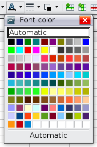
To choose a font color, click the arrow next to the Font Color icon to display a color palette. Click on the required color.

(To define custom colors, use Tools → Options → LibreOffice → Colors. See Chapter 14 for more information.)

To specify the language of the cell (useful because it allows different languages to exist in the same document and be spell checked correctly), use the Font tab of the Format Cells dialog. See Chapter 4 for more information.

Choosing font effects

The Font Effects tab (Figure 18) of the Format Cells dialog offers more font options.

Overlining and underlining

You can choose from a variety of overlining and underlining options (solid lines, dots, short and long dashes, in various combinations) and the color of the line.

Strikethrough

The strikethrough options include lines, slashes, and Xs.

Relief

The relief options are embossed (raised text), engraved (sunken text), outline, and shadow.

Setting cell alignment and orientation

Some of the cell alignment and orientation icons are not shown by default on the Formatting toolbar. To show them, click on the small arrow at the right-hand end of the toolbar and select them from the list of icons.

Some of the alignment and orientation icons are available only if you have Asian or CTL (Complex Text Layout) languages enabled (in Tools → Options → Language Settings → Languages). If you choose an unavailable icon from the list, it does not appear on the toolbar.

For more control and other choices, use the Alignment tab (Figure 13) of the Format Cells dialog to set the horizontal and vertical alignment and rotate the text. If you have Asian languages enabled, then the Text orientation section shows an extra option (labeled Asian layout mode) under the Vertically stacked option, as shown in Figure 20.

The difference in results between having Asian layout mode on or off is shown in Figure 21.

Formatting the cell borders

To quickly choose a line style and color for the borders of a cell, click the small arrows next to the Line Style and Line Color icons on the Formatting toolbar. If the Line Style and Line Color icons are not displayed in the formatting toolbar, select the down arrow on the right side of the bar, then select Visible Buttons. In each case, a palette of choices is displayed.

For more control, including the spacing between the cell borders and the text, use the Borders tab of the Format Cells dialog. There you can also define a shadow. See Chapter 4 for details.

Formatting the cell background

To quickly choose a background color for a cell, click the small arrow next to the Background Color icon on the Formatting toolbar. A palette of color choices, similar to the Font Color palette, is displayed.

(To define custom colors, use Tools → Options → LibreOffice → Colors. See Chapter 14 for more information.)

You can also use the Background tab of the Format Cells dialog. See Chapter 4 for details.

Autoformatting cells and sheets

You can use the AutoFormat feature to quickly apply a set of cell formats to a sheet or a selected cell range.

1. Select the cells that you want to format, including the column and row headers.

2. Choose Format → AutoFormat.

3. To select which properties (number format, font, alignment, borders, pattern, autofit width and height) to include in an AutoFormat, click More. Select or deselect the required options. Click OK.

If you do not see any change in color of the cell contents, choose View → Value Highlighting from the menu bar. This function only affects cells with numerical data.

Defining a new AutoFormat

You can define a new AutoFormat that is available to all spreadsheets.

1. Format a sheet.

2. Choose Edit → Select All.

3. Choose Format → AutoFormat. The Add button is now active.

4. Click Add.

5. In the Name box of the Add AutoFormat dialog, type a meaningful name for the new format.

6. Click OK to save. The new format is now available in the Format list in the AutoFormat dialog.

Formatting spreadsheets using themes

Calc comes with a predefined set of formatting themes that you can apply to your spreadsheets.

It is not possible to add themes to Calc, and they cannot be modified. However, you can modify their styles after you apply them to a spreadsheet.

To apply a theme to a spreadsheet:

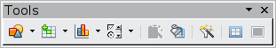
1. Click the Choose Themes icon in the Tools toolbar. If this toolbar is not visible, you can show it using View → Toolbars → Tools. The Theme Selection dialog appears. This dialog lists the available themes for the whole spreadsheet.

2. In the Theme Selection dialog, select the theme that you want to apply to the spreadsheet. As soon as you select a theme, some of the properties of the custom styles are applied to the open spreadsheet and are immediately visible.

3. Click OK. If you wish, you can now go to the Styles and Formatting window to modify specific styles. These modifications do not change the theme; they only change the appearance of this specific spreadsheet document.

Using conditional formatting

You can set up cell formats to change depending on conditions that you specify. For example, in a table of numbers, you can show all the values above the average in green and all those below the average in red.

Conditional formatting depends upon the use of styles. If you are not familiar with styles, please refer to Chapter 4. An easy way to set up the required styles is to format a cell the way you want it and click the New Style from Selection icon in the Styles and Formatting window.

After the styles are set up, here is how to use them.

1. In your spreadsheet, select the cells to which you want to apply conditional formatting.

2. Choose Format → Conditional Formatting from the menu bar.

3. On the Conditional Formatting dialog (Figure 23), enter the conditions. Click OK to save. The selected cells are now formatted in the relevant style.

Cell value is / Formula is

Specifies whether conditional formatting is dependent on a cell value or on a formula. If you select cell value is, the Cell Value Condition box is displayed, as shown in the example. Here you can choose from conditions including less than, greater than, between, and others.

Parameter field

Enter a reference, value, or formula in the parameter field, or in both parameter fields if you have selected a condition that requires two parameters. You can also enter formulas containing relative references.

Cell style

Choose the cell style to be applied if the specified condition matches. The style must have been defined previously.

See the Help for more information and examples of use.

To apply the same conditional formatting later to other cells:

1. Select one of the cells that has been assigned conditional formatting.

2. Copy the cell to the clipboard.

3. Select the cells that are to receive this same formatting.

4. Choose Edit → Paste Special.

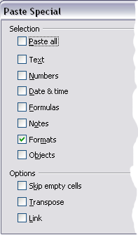
5. On the Paste Special dialog, in the Selection area, select only the Formats option. Make sure all other options are not selected. Click OK.

Hiding and showing data

When elements are hidden, they are neither visible nor printed, but can still be selected for copying if you select the elements around them. For example, if column B is hidden, it is copied when you select columns A and C. When you need a hidden element again, you can reverse the process, and show the element.

To hide or show sheets, rows, and columns, use the options on the Format menu or the right-click (context) menu. For example, to hide a row, first select the row, and then choose Format → Row → Hide (or right-click and choose Hide).

To hide or show selected cells, choose Format → Cells from the menu bar (or right-click and choose Format Cells). On the Format Cells dialog, go to the Cell Protection tab.

Outline group controls

If you are continually hiding and showing the same cells, you can simplify the process by creating outline groups, which add a set of controls for hiding and showing the cells in the group that are quick to use and always available.

If the contents of cells fall into a regular pattern, such as four cells followed by a total, then you can use Data → Group and Outline → AutoOutline to have Calc add outline controls based on the pattern. Otherwise, you can set outline groups manually by selecting the cells for grouping, then choosing Data → Group and Outline → Group. On the Group dialog, you can choose whether to group the selected cells by rows or columns.

When you close the dialog, the outline group controls are visible between either the row or column headers and the edges of the editing window. The controls resemble the tree-structure of a file-manager in appearance, and can be hidden by selecting Data → Group and Outline → Hide Details. They are strictly for online use, and do not print.

The basic outline controls have plus or minus signs at the start of the group to show or hide hidden cells. However, if outline groups are nested, the controls have numbered buttons for hiding the different levels.

If you no longer need a group, place the mouse cursor in any cell in it and select Data → Group and Outline → Ungroup. To remove all groups on a sheet, select Data → Group and Outline → Remove.

Filtering which cells are visible

A filter is a list of conditions that each entry has to meet in order to be displayed. You can set three types of filters from the Data → Filter sub-menu.

Automatic filters add a drop-down list to the top row of a column that contains commonly used filters. They are quick and convenient and almost as useful with text as with numbers, because the list includes every unique entry in the selected cells.

In addition to these unique entries, automatic filters include the option to display all entries, the ten highest numerical values, and all cells that are empty or not empty, as well as a standard filter that you can customize (see below). However, they are somewhat limited. In particular, they do not allow regular expressions, so you cannot use them to display cell contents that are similar but not identical.

Standard filters are more complex than automatic filters. You can set as many as three conditions as a filter, combining them with the operators AND and OR. Standard filters are mostly useful for numbers, although a few of the conditional operators, such as = and < > can also be used for text.

Other conditional operators for standard filters include options to display the largest or smallest values, or a percentage of them. Useful in themselves, standard filters take on added value when they are used to further refine automatic filters.

Advanced filters are structured similarly to standard filters. The differences are that advanced filters are not limited to three conditions, and their criteria are not entered in a dialog. Instead, advanced filters are entered in a blank area of a sheet, then referenced by the advanced filter tool in order to apply them.

Sorting records

Sorting rearranges the visible cells on the sheet. In Calc, you can sort by up to three criteria, which are applied one after another. Sorts are handy when you are searching for a particular item, and become even more powerful after you have filtered data.

In addition, sorting is often useful when you add new information. When a list is long, it is usually easier to add new information at the bottom of the sheet, rather than inserting rows in the proper places. After you have added the information, you can sort it to update the sheet.

Highlight the cells to be sorted, then select Data → Sort to open the Sort dialog (Figure 26) or click the Sort Ascending or Sort Descending toolbar buttons. Using the dialog, you can sort the selected cells using up to three columns, in either ascending (A-Z, 1-9) or descending (Z-A, 9-1) order.

On the Options tab of the Sort dialog (Figure 27), you can choose the following options.

Case sensitive

If two entries are otherwise identical, one with an upper case letter is placed before one with a lower case letter in the same position if the sort is descending; if the sort is ascending, then the entry with an upper case letter is placed after one with a lower case letter in the same position.

Range contains column labels

Does not include the column heading in the sort.

Include formats

A cell's formatting is moved with its contents. If formatting is used to distinguish different types of cells, then use this option.

Copy sort results to

Sets a spreadsheet address to which to copy the sort results. If a range is specified that does not have the necessary number of cells, then cells are added. If a range contains cells that already have content, then the sort fails.

Custom sort order

Select the box, then choose from the drop-down list one of the sort orders defined in Tools → Options → LibreOffice Calc → Sort Lists.

Direction

Sets whether rows or columns are sorted. The default is to sort by columns unless the selected cells are in a single column.

Finding and replacing in Calc

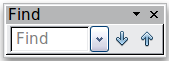
Calc has two ways to find text within a document: the Find toolbar for fast text searching and the Find & Replace dialog.

Using the Find toolbar

The Find toolbar is located by default on the right-hand end of the Standard toolbar. You can hide or show the Find toolbar using View → Toolbars → Find.

Type a search term in the Find box, and then click the Find Next (down-arrow) or Find Previous (up-arrow) button. To find other occurrences of the same term, continue clicking the button.

Using the Find & Replace dialog

To display the Find & Replace dialog (Figure 28), use the keyboard shortcut Control+F or choose Edit → Find & Replace from the menu bar.

In spreadsheet documents you can search for text, formulas, and styles. You can navigate from one occurrence to the next using Find, or you can highlight all matching cells at once using Find All, then apply another format or replace the cell contents by other content.

Text and numbers in cells may have been entered directly or may be the result of a calculation. The search method you use depends on the type of data you are searching for.

By default, Calc searches the current sheet. To search through all sheets of the document, click More Options, then select Search in all sheets option.

Finding and replacing formulas or values

You can use the Find & Replace dialog to search in formulas or in the displayed values that result from a calculation.

1. To open the Find & Replace dialog, use the keyboard shortcut Control+F or select Edit → Find & Replace.

2. Click More Options to expand the dialog.

3. Select Formulas or Values in the Search in drop-down list.

• Formulas finds parts of the formulas.

• Values finds the results of the calculations.

4. Type the text you want to find in the Search for box.

5. To replace the text with different text, type the new text in the Replace with box.

6. When you have set up your search, click Find. To replace text, click Replace instead.

Finding and replacing text

1. Open the Find & Replace dialog, click More Options to expand the dialog, and select Values or Notes in the Search in drop-down list.

2. Type the text you want to find in the Search for box.

3. To replace the text with different text, type the new text in the Replace with box.

4. Click Find, Find All, Replace, or Replace All.

When you click Find, Calc selects the next cell that contains your text. You can edit the text, then click Find again to advance to the next found cell. If you closed the dialog, you can press Ctrl+Shift+F to find the next cell without opening the dialog.

When you click Find All, Calc selects all cells that contain your entry. Now you can, for example, apply a cell style to all of them at once.

Finding and replacing cell styles

To quickly change all the paragraphs of one (unwanted) style to another (preferred) style:

1. On the expanded Find & Replace dialog, select Search for Styles. The Search for and Replace with boxes now contain a list of styles.

2. Select the styles you want to search for and replace.

3. Click Find, Find All, Replace, or Replace All.

Using wildcards (regular expressions)

Wildcards (also known as regular expressions) are combinations of characters that instruct LibreOffice how to search for something. Regular expressions are very powerful but not very intuitive. They can save time and effort by combining multiple finds into one.

To use wildcards and regular expressions when searching and replacing:

1. On the Find & Replace dialog, click More Options to see more choices. On this expanded dialog, select the Regular expressions option.

2. Type the search text, including the wildcards, in the Search for box and the replacement text (if any) in the Replace with box.

3. Click Find, Find All, Replace, or Replace All (not recommended).

The following points may be of interest to Calc users:

• In Calc, regular expressions are applied separately to each cell. This means that a search for r.d will match red in cell A1 but will not match r in cell A2 and d (or ed) in cell A3. (The regular expression r.d means the system will try to match r followed by any other character followed by d.)

• When a match is found, the entire cell is highlighted but only the text found will be replaced. For example, searching for brown will result in highlighting a cell containing redbrown clay, and choosing nothing in the Replace with box leaves the cell containing red clay.

• If Find is used twice in a row, and the second time the Current selection only box is activated, then the second search will evaluate the whole of each selected cell, not just the strings that caused the cells to be selected in the first search. For example, searching for joh?n, then activating Current selection only and searching for sm.th will find cells containing Jon Smith and Smythers, Johnathon.

• If a cell contains a hard line break (entered by Ctrl+Enter), it may be found by using the regular expression \n. For example, if a cell contains red [hard line break] clay then searching for d\nc and entering nothing in the Replace with box leaves the cell containing relay.

• The hard line break acts to mark “end of text” (similar to “end of paragraph” in Writer), found by the regular expression special character $, in addition to the end of text in the cell. For example, if a cell contains red [hard line break] clay then a search for d$ replacing with al leaves the cell with real [hard line break] clay. Note that with this syntax the hard line break is not replaced.

• Using \n in the Replace with box will replace with the literal characters \n, not a hard line break.

• The Find & Replace dialog has an option to search within formulas, values, or notes. This option applies to any search, not just one using regular expressions. Searching with the Formulas option for SUM would find a cell containing the formula =SUM(A1:A6) as well as a cell containing the simple text SUMMARY.

• Searching for the regular expression ^$ will not find empty cells. This is intentional, to avoid performance issues when selecting a huge number of cells. Note that empty cells will not be found even if you are only searching a selection.

• Finding cell contents using the regular expression .+ (or similar) and replacing them with & effectively re-enters the cell contents without any formatting. This technique can be used to remove formatting automatically applied by Calc when importing data from the clipboard or from badly formatted files. For example, to convert text strings consisting of digits into actual numbers, first format the cells as numbers and then perform the search and replace.

See Chapter 7, Using Formulas and Functions, for the use of regular expressions within formulas.