Getting Started Guide
Chapter
5
Getting Started with Calc
Using Spreadsheets in LibreOffice
This document is Copyright © 2010 by its contributors as listed below. You may distribute it and/or modify it under the terms of either the GNU General Public License (http://www.gnu.org/licenses/gpl.html), version 3 or later, or the Creative Commons Attribution License (http://creativecommons.org/licenses/by/3.0/), version 3.0 or later.
All trademarks within this guide belong to their legitimate owners.
Contributors
Ron
Faile Jr.
Hal Parker
Feedback
Please direct any comments or suggestions about this document to: documentation@libreoffice.org
Acknowledgments
This chapter is based on the Chapter 5 of Getting Started with OpenOffice.org. The contributors to that chapter are:
Richard
Barnes Richard Detwiler
John Kane Peter Kupfer
Joe
Sellman Jean Hollis Weber
Linda Worthington Michele Zarri
Publication date and software version
Published 30 December 2010. Based on LibreOffice 3.3.
Some keystrokes and menu items are different on a Mac from those used in Windows and Linux. The table below gives some common substitutions for the instructions in this chapter. For a more detailed list, see the application Help.
|
Windows/Linux |
Mac equivalent |
Effect |
|
Tools → Options menu selection |
LibreOffice → Preferences |
Access setup options |
|
Right-click |
Control+click |
Opens a context menu |
|
Ctrl (Control) |
z (Command) |
Used with other keys |
|
F5 |
Shift+z+F5 |
Opens the Navigator |
|
F11 |
z+T |
Opens the Styles & Formatting window |
Contents
Spreadsheets, sheets and cells 5
Parts of the main Calc window 6
Opening and saving CSV files 8
Navigating within spreadsheets 10
Selecting items in a sheet or spreadsheet 14
Working with columns and rows 16
Entering data using the keyboard 21
Deactivating automatic changes 22
Using the Fill tool on cells 23
Sharing content between sheets 26
Replacing all the data in a cell 27
Changing part of the data in a cell 27
Formatting multiple lines of text 28
Shrinking text to fit the cell 29
Formatting the cell borders 31
Formatting the cell background 31
Autoformatting cells and sheets 31
Formatting spreadsheets using themes 32
Using conditional formatting 33
Filtering which cells are visible 34
Selecting the page order, details, and scale 36
Calc is the spreadsheet component of LibreOffice. You can enter data (usually numerical) in a spreadsheet and then manipulate this data to produce certain results.
Alternatively you can enter data and then use Calc in a ‘What if...’ manner by changing some of the data and observing the results without having to retype the entire spreadsheet.
Other features provided by Calc include:
Functions, which can be used to create formulas to perform complex calculations on data
Database functions, to arrange, store, and filter data
Dynamic charts; a wide range of 2D and 3D charts
Macros, for recording and executing repetitive tasks
Ability to open, edit, and save Microsoft Excel spreadsheets
Import and export of spreadsheets in multiple formats, including HTML, CSV, PDF, and PostScript
|
Note |
If you want to use macros written in Microsoft Excel using the VBA macro code in LibreOffice, you must first edit the code in the LibreOffice Basic IDE editor. See Chapter 13, Getting Started with Macros, in this book and Chapter 12 in the Calc Guide. |
Spreadsheets, sheets and cells
Calc works with documents called spreadsheets. Spreadsheets consist of a number of individual sheets, each sheet containing cells arranged in rows and columns. A particular cell is identified by its row number and column letter.
Cells hold the individual elements—text, numbers, formulas, and so on—that make up the data to display and manipulate.
Each spreadsheet can have many sheets, and each sheet can have many individual cells. In Calc 3.3, each sheet can have a maximum of 1,048,576 rows and 1024 columns.
When Calc is started, the main window looks similar to Figure 1.
The Title bar, located at the top, shows the name of the current spreadsheet. When the spreadsheet is newly created, its name is Untitled X, where X is a number. When you save a spreadsheet for the first time, you are prompted to enter a name of your choice.
Under the Title bar is the Menu bar. When you choose one of the menus, a submenu appears with other options. You can modify the Menu bar, as discussed in Chapter 14, Customizing LibreOffice.
Three toolbars are located under the Menu bar by default: the Standard toolbar, the Formatting toolbar, and the Formula Bar.
The icons (buttons) on these toolbars provide a wide range of common commands and functions. You can also modify these toolbars, as discussed in Chapter 14, Customizing LibreOffice.
In the Formatting toolbar, the three boxes on the left are the Apply Style, Font Name, and Font Size lists. They show the current setting for the selected cell or area. (The Apply Style list may not be visible by default.) Click the down-arrow to the right of each box to open the list.
On the left hand side of the Formula bar is a small text box, called the Name Box, with a letter and number combination in it, such as D7. This combination, called the cell reference, is the column letter and row number of the selected cell.
To the right of the Name box are the the Function Wizard, Sum, and Function buttons.
Clicking the Function Wizard button opens a dialog from which you can search through a list of available functions This can be very useful because it also shows how the functions are formatted.
In a spreadsheet the term function covers much more than just mathematical functions. See Chapter 7 in the Calc Guide for more details.
Clicking the Sum button inserts a formula into the current cell that totals the numbers in the cells above the current cell. If there are no numbers above the current cell, then the cells to the left are placed in the Sum formula.
Clicking the Function button inserts an equals (=) sign into the selected cell and the Input line, enabling the cell to accept a formula.
When
you enter new data into a cell, the Sum and Equals buttons change to
Cancel
and Accept
buttons
![]() .
.
The contents of the current cell (data, formula, or function) are displayed in the Input line, which forms the remainder of the Formula Bar. You can edit the contents of the current cell on the Input line or in the cell itself. To edit on the Input line, click in the line, then type your changes. To edit within the current cell, just double-click the cell.
The main section of the screen displays the cells in the form of a grid, with each cell being at the intersection of a column and a row.
At the top of the columns and at the left end of the rows are a series of gray boxes containing letters and numbers. These are the column and row headers. The columns start at A and go on to the right, and the rows start at 1 and go down.
These column and row headers form the cell references that appear in the Name Box on the Formula Bar (Figure 3). You can turn these headers off by selecting View → Column & Row Headers.
At the bottom of the grid of cells are the sheet tabs. These tabs enable access to each individual sheet, with the visible (active) sheet having a white tab. You can choose colors for the different sheet tabs.
Clicking on another sheet tab displays that sheet, and its tab turns white. You can also select multiple sheet tabs at once by holding down the Control key while you click the names.
At the very bottom of the Calc window is the status bar, which provides information about the spreadsheet and convenient ways to quickly change some of its features. Most of the fields are similar to those in other components of LibreOffice; see Chapter 1, Introducing LibreOffice, in this book and Chapter 1, Introducing Calc, in the Calc Guide.
Chapter 1, Introducing LibreOffice, includes instructions on starting new Calc documents, opening existing documents, and saving documents.
A special case for Calc is opening and saving comma-separated-values (CSV) files, which are text files that contain the cell contents of a single sheet. Each line in a CSV file represents a row in a spreadsheet. Commas, semicolons, or other characters are used to separate the cells. Text is entered in quotation marks, numbers are entered without quotation marks.
To open a CSV file in Calc:
Choose File → Open.
Locate the CSV file that you want to open.
If the file has a *.csv extension, select the file and click Open.
If the file has another extension (for example, *.txt), select the file, select Text CSV (*csv;*txt;*xls) in the File type box (scroll down into the spreadsheet section to find it) and then click Open.
On the Text Import dialog (Figure 6), select the Separator options to divide the text in the file into columns.
You can preview the layout of the imported data at the bottom of the dialog. Right-click a column in the preview to set the format or to hide the column.
If the CSV file uses a text delimiter character that is not in the Text delimiter list, click in the box, and type the character.
Click OK to open the file.
To save a spreadsheet as a comma separate value (CSV) file:
Choose File → Save As.
In the File name box, type a name for the file.
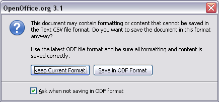
In the File type list, select Text CSV (.csv) and click Save.
You may see the message box shown below. Click Keep Current Format.
In the Export of text files dialog, select the options you want and then click OK.
Navigating within spreadsheets
Calc provides many ways to navigate within a spreadsheet from cell to cell and sheet to sheet. You can generally use the method you prefer.
Using the mouse
Place the mouse pointer over the cell and click.
Using a cell reference
Click on the little inverted black triangle just to the right of the Name Box (Figure 3). The existing cell reference will be highlighted. Type the cell reference of the cell you want to go to and press Enter. Or just click into the Name box, backspace over the existing cell reference and type in the cell reference you want and press Enter.
Using the Navigator
To
open the Navigator, click its icon
![]() on the Standard toolbar, or press F5,
or choose View
→
Navigator on the
Menu bar, or double-click on the Sheet Sequence Number
on the Standard toolbar, or press F5,
or choose View
→
Navigator on the
Menu bar, or double-click on the Sheet Sequence Number
![]() in the Status Bar.
Type the cell reference into the top two fields,
labeled Column and Row, and press Enter.
In Figure 8 the Navigator would select cell A7.
in the Status Bar.
Type the cell reference into the top two fields,
labeled Column and Row, and press Enter.
In Figure 8 the Navigator would select cell A7.
You can dock the Navigator to either side of the main Calc window or leave it floating. (To dock or float the Navigator, hold down the Control key and double-click in an empty area near the icons in the Navigator dialog.)
The Navigator displays lists of all the objects in a document, grouped into categories. If an indicator (plus sign or arrow) appears next to a category, at least one object of this kind exists. To open a category and see the list of items, click on the indicator.
To
hide the list of categories and show only the icons at the top, click
the Contents
icon
![]() .
Click this icon again to show the list.
.
Click this icon again to show the list.
In the spreadsheet, one cell normally has a black border. This black border indicates where the focus is (see Figure 9). If a group of cells is selected, they are highlighted in a light blue color, with the focus cell having a black border.
Using the mouse
To move the focus using the mouse, simply move the mouse pointer to the cell where you want the focus to be and click the left mouse button. This changes the focus to the new cell. This method is most useful when the two cells are a large distance apart.
Using the Tab and Enter keys
Pressing Enter or Shift+Enter moves the focus down or up, respectively.
Pressing Tab or Shift+Tab moves the focus to the right or to the left, respectively.
Using the arrow keys
Pressing the arrow keys on the keyboard moves the focus in the direction of the arrows.
Using Home, End, Page Up and Page Down
Home moves the focus to the start of a row.
End moves the focus to the column furthest to the right that contains data.
Page Down moves the display down one complete screen and Page Up moves the display up one complete screen.
Combinations of Control and Alt with Home, End, Page Down, Page Up, and the cursor keys move the focus of the current cell in other ways. See the Help or Appendix A, Keyboard Shortcuts, in the Calc Guide for details.
|
Tip |
Use one of the four Alt+Arrow key combinations to resize a cell. |
Customizing the Enter key
You can customize the direction in which the Enter key moves the focus, by selecting Tools → Options → LibreOffice Calc → General.
The four choices for the direction of the Enter key are shown on the right hand side of Figure 10. It can move the focus down, right, up, or left. Depending on the file being used or on the type of data being entered, setting a different direction can be useful.
The Enter key can also be used to switch into and out of editing mode. Use the first two options under Input settings in Figure 10 to change the Enter key settings.

Each sheet in a spreadsheet is independent of the others, though they can be linked with references from one sheet to another. There are three ways to navigate between different sheets in a spreadsheet.
Using the Navigator
When the Navigator is open (Figure 8), double-clicking on any of the listed sheets selects the sheet.
Using the keyboard
Pressing Control+Page Down moves one sheet to the right and pressing Control+Page Up moves one sheet to the left.
Using the mouse
Clicking on one of the sheet tabs at the bottom of the spreadsheet selects that sheet.
If you have a lot of sheets, then some of the sheet tabs may be hidden behind the horizontal scroll bar at the bottom of the screen. If this is the case, then the four buttons at the left of the sheet tabs can move the tabs into view. Figure 11 shows how to do this.
Notice that the sheets here are not numbered in order. Sheet numbering is arbitrary; you can name a sheet as you wish.
|
Note |
The sheet tab arrows that appear in Figure 11 only appear if you have some sheet tabs that are hidden by the horizontal scrollbar. Otherwise, they will appear faded as in Figure 1. |
Selecting items in a sheet or spreadsheet
Cells can be selected in a variety of combinations and quantities.
Single cell
Left-click in the cell. The result will look like the left side of Figure 9. You can verify your selection by looking in the Name box.
Range of contiguous cells
A range of cells can be selected using the keyboard or the mouse.
To select a range of cells by dragging the mouse:
Click in a cell.
Press and hold down the left mouse button.
Move the mouse around the screen.
Once the desired block of cells is highlighted, release the left mouse button.
To select a range of cells without dragging the mouse:
Click in the cell which is to be one corner of the range of cells.
Move the mouse to the opposite corner of the range of cells.
Hold down the Shift key and click.
To select a range of cells without using the mouse:
Select the cell that will be one of the corners in the range of cells.
While holding down the Shift key, use the cursor arrows to select the rest of the range.
The result of any of these methods looks like the right side of Figure 9.
|
Tip |
You can also directly select a range of cells using the Name box. Click into the Name Box as described in “Using a cell reference” on page 10. To select a range of cells, enter the cell reference for the upper left-hand cell, followed by a colon (:), and then the lower right-hand cell reference. For example, to select the range that would go from A3 to C6, you would enter A3:C6. |
Range of non-contiguous cells
Select the cell or range of cells using one of the methods above.
Move the mouse pointer to the start of the next range or single cell.
Hold down the Control key and click or click-and-drag to select a range.
Repeat as necessary.
Entire columns and rows can be selected very quickly in LibreOffice.
Single column or row
To select a single column, click on the column identifier letter (see Figure 1).
To select a single row, click on the row identifier number.
Multiple columns or rows
To select multiple columns or rows that are contiguous:
Click on the first column or row in the group.
Hold down the Shift key.
Click the last column or row in the group.
To select multiple columns or rows that are not contiguous:
Click on the first column or row in the group.
Hold down the Control key.
Click on all of the subsequent columns or rows while holding down the Control key.
Entire sheet
To select the entire sheet, click on the small box between the A column header and the 1 row header.
You can also press Control+A to select the entire sheet.
You can select either one or multiple sheets. It can be advantageous to select multiple sheets at times when you want to make changes to many sheets at once.
Single sheet
Click on the sheet tab for the sheet you want to select. The active sheet becomes white (see Figure 13).
Multiple contiguous sheets
To select multiple contiguous sheets:
Click on the sheet tab for the first desired sheet.
Move the mouse pointer over the sheet tab for the last desired sheet.
Hold down the Shift key and click on the sheet tab.
All the tabs between these two sheets will turn white. Any actions that you perform will now affect all highlighted sheets.
Multiple non-contiguous sheets
To select multiple non-contiguous sheets:
Click on the sheet tab for the first sheet.
Move the mouse pointer over the second sheet tab.
Hold down the Control key and click on the sheet tab.
Repeat as necessary.
The selected tabs will turn white. Any actions that you perform will now affect all highlighted sheets.
All sheets
Right-click any one of the sheet tabs and choose Select All Sheets from the pop-up menu.
Columns and rows can be inserted individually or in groups.
|
Note |
When you insert a single new column, it is inserted to the left of the highlighted column. When you insert a single new row, it is inserted above the highlighted row. Cells in the new columns or rows are formatted like the corresponding cells in the column or row before (or to the left of) which the new column or row is inserted. |
Single column or row
Using the Insert menu:
Select the cell, column or row where you want the new column or row inserted.
Choose either Insert → Columns or Insert → Rows.
Using the mouse:
Select the cell, column or row where you want the new column or row inserted.
Right-click the header of the column or row.
Choose Insert Rows or Insert Columns.
Multiple columns or rows
Multiple columns or rows can be inserted at once rather than inserting them one at a time.
Highlight the required number of columns or rows by holding down the left mouse button on the first one and then dragging across the required number of identifiers.
Proceed as for inserting a single column or row above.
Columns and rows can be deleted individually or in groups.
Single column or row
A single column or row can only be deleted by using the mouse:
Select the column or row to be deleted.
Right-click on the column or row header.
Select Delete Columns or Delete Rows from the pop-up menu.
Multiple columns or rows
Multiple columns or rows can be deleted at once rather than deleting them one at a time.
Highlight the required number of columns or rows by holding down the left mouse button on the first one and then dragging across the required number of identifiers.
Proceed as for deleting a single column or row above.
Like any other Calc element, sheets can be inserted, deleted, and renamed.
There
are several ways to insert a new sheet. The fastest method is to
click on the Add Sheet button
![]() .
This inserts one new sheet at that point, without opening the Insert
Sheet dialog.
.
This inserts one new sheet at that point, without opening the Insert
Sheet dialog.
Use one of the other methods to insert more than one sheet, to rename the sheet at the same time, or to insert the sheet somewhere else in the sequence. The first step for these methods is to select the sheet that the new sheet will be inserted next to. Then use any of the following options.
Choose Insert → Sheet from the menu bar.
Right-click on a sheet tab and choose Insert Sheet.
Click in an empty space at the end of the line of sheet tabs.
Each method will open the Insert Sheet dialog (Figure 14). Here you can select whether the new sheet is to go before or after the selected sheet and how many sheets you want to insert. If you are inserting only one sheet, there is the opportunity to give the sheet a name.
Sheets can be deleted individually or in groups.
Single sheet
Right-click on the tab of the sheet you want to delete and choose Delete Sheet from the pop up menu, or chose Edit → Sheet → Delete from the menu bar.
Multiple sheets
To delete multiple sheets, select them as described earlier, then either right-click over one of the tabs and select Delete Sheet from the pop-up menu, or choose Edit → Sheet → Delete from the menu bar.
The default name for the a new sheet is SheetX, where X is a number. While this works for a small spreadsheet with only a few sheets, it becomes awkward when there are many sheets.
To give a sheet a more meaningful name, you can:
Enter the name in the Name box when you create the sheet, or
Right-click on a sheet tab and choose Rename Sheet from the pop-up menu; replace the existing name with one of your choosing.
Double-click on a sheet tab to pop up the Rename Sheet dialog.
|
Note |
Sheet names must start with either a letter or a number. Apart from the first character of the sheet name, allowed characters are letters, numbers, spaces, and the underline character. Attempting to rename a sheet with an invalid name will produce an error message. |
Use the zoom function to change the view to show more or fewer cells in the window. For more about zoom, see Chapter 1, Introducing LibreOffice, in this book.
Freezing locks a number of rows at the top of a spreadsheet or a number of columns on the left of a spreadsheet or both. Then when scrolling around within the sheet, any frozen columns and rows remain in view.
Figure 15 shows some frozen rows and columns. The heavier horizontal line between rows 3 and 14 and the heavier vertical line between columns C and H denote the frozen areas. Rows 4 through 13 and columns D through G have been scrolled off the page. The first three rows and columns remained because are frozen into place.
You can set the freeze point at a row, a column, or both a row and a column as in Figure 15.
Freezing single rows or columns
Click on the header for the row below where you want the freeze or for the column to the right of where you want the freeze.
Choose Window → Freeze.
A dark line appears, indicating where the freeze is put.
Freezing a row and a column
Click into the cell that is immediately below the row you want frozen and immediately to the right of the column you want frozen.
Choose Window → Freeze.
Two lines appear on the screen, a horizontal line above this cell and a vertical line to the left of this cell. Now as you scroll around the screen, everything above and to the left of these lines will remain in view.
Unfreezing
To unfreeze rows or columns, choose Window → Freeze. The check mark by Freeze will vanish.
Another way to change the view is by splitting the window, also known as splitting the screen. The screen can be split either horizontally or vertically or both. You can therefore have up to four portions of the spreadsheet in view at any one time.
Why would you want to do this? Imagine you have a large spreadsheet and one of the cells has a number in it which is used by three formulas in other cells. Using the split screen technique, you can position the cell containing the number in one section and each of the cells with formulas in the other sections. Then you can change the number in the cell and watch how it affects each of the formulas.
Splitting the screen horizontally
To split the screen horizontally:
Move the mouse pointer into the vertical scroll bar, on the right-hand side of the screen, and place it over the small button at the top with the black triangle. Immediately above this button you will see a thick black line.
Move the mouse pointer over this line and it turns into a line with two arrows.
Hold down the left mouse button. A gray line appears, running across the page. Drag the mouse downwards and this line follows.
Release the mouse button and the screen splits into two views, each with its own vertical scroll bar. You can scroll the upper and lower parts independently.
Notice in Figure 16, the Beta and the A0 values are in the upper part of the window and other calculations are in the lower part. Thus you can make changes to the Beta and A0 values and watch their affects on the calculations in the lower half of the window.
|
Tip |
You can also split the screen using a menu command. Click in a cell immediately below and to the right of where you wish the screen to be split, and choose Window → Split. |
Splitting the screen vertically
To split the screen vertically:
Move the mouse pointer into the horizontal scroll bar at the bottom of the screen and place it over the small button on the right with the black triangle. Immediately to the right of this button is a thick black line.
Move the mouse pointer over this line and it turns into a line with two arrows.
Hold down the left mouse button, and a gray line appears, running up the page. Drag the mouse to the left and this line follows.
Release the mouse button and the screen is split into two views, each with its own horizontal scroll bar. You can scroll the left and right parts of the window independently.
Removing split views
To remove a split view, do any of the following:
Double-click on each split line.
Click on and drag the split lines back to their places at the ends of the scroll bars.
Choose Window → Split to remove all split lines at the same time.
Entering data using the keyboard
Most data entry in Calc can be accomplished using the keyboard.
Click in the cell and type in the number using the number keys on either the main keyboard or the numeric keypad.
To enter a negative number, either type a minus (–) sign in front of it or enclose it in parentheses (brackets), like this: (1234).
By default, numbers are right-aligned and negative numbers have a leading minus symbol.
|
Note |
If a number beginning with 0 is entered in to a cell, Calc will drop the 0 (for example 01234 becomes 1234). |
To enter a number and retain the leading 0, right-click on the cell and choose Format Cells → Numbers. In the Format Cells dialog, under Options select the required number of Leading zeros.
The number selected for leading zeros needs to be one higher than the digits in a number. For example, if the number is 1234, the number entered for the leading zero will be 5.
Click in the cell and type the text. Text is left-aligned by default.
A number can be entered as text to preserve a leading zero by entering an apostrophe before the number, like this: '01481.
The data is now regarded as text by Calc and displayed exactly as entered. Typically, formulas will treat the entry as a zero and functions will ignore it. Take care that the cell containing the number is not used in a formula.
|
Note |
If “smart quotes” are used for apostrophes, the apostrophe remains visible in the cell. To choose the type of apostrophe, use Tools → AutoCorrect → Custom Quotes. The selection of the apostrophe type affects both Calc and Writer. |
Select the cell and type the date or time. You can separate the date elements with a slant (/) or a hyphen (–) or use text such as 15 Oct 10. Calc recognizes a variety of date formats. You can separate time elements with colons such as 10:43:45.
Deactivating automatic changes
Calc automatically applies many changes during data input, unless you deactivate those changes. You can also immediately undo any automatic changes with Ctrl+Z.
AutoCorrect changes
Automatic correction of typing errors, replacement of straight quotation marks by curly (custom) quotes, and starting cell content with an uppercase (capital letter) are controlled by Tools → AutoCorrect Options. Go to the Custom Quotes, Options, or Replace tabs to deactivate any of the features that you do not want. On the Replace tab, you can also delete unwanted word pairs and add new ones as required.
AutoInput
When you are typing in a cell, Calc automatically suggests matching input found in the same column. To turn the AutoInput on and off, set or remove the check mark in front of Tools → Cell Contents → AutoInput.
Automatic date conversion
Calc automatically converts certain entries to dates. To ensure that an entry that looks like a date is interpreted as text, type an apostrophe at the beginning of the entry. The apostrophe is not displayed in the cell.
Entering data into a spreadsheet can be very labor-intensive, but Calc provides several tools for removing some of the drudgery from input.
The most basic ability is to drag and drop the contents of one cell to another with a mouse. Calc also includes several other tools for automating input, especially of repetitive material. They include the Fill tool, selection lists, and the ability to input information into multiple sheets of the same document.
At its simplest, the Fill tool is a way to duplicate existing content. Start by selecting the cell to copy, then drag the mouse in any direction (or hold down the Shift key and click in the last cell you want to fill), and then choose Edit → Fill and the direction in which you want to copy: Up, Down, Left or Right.
|
Caution
|
Choices that are not available are grayed out, but you can still choose the opposite direction from what you intend, which could cause you to overwrite cells accidentally. |
|
Tip |
A shortcut way to fill cells is to grab the “handle” in the lower right-hand corner of the cell and drag it in the direction you want to fill. If the cell contains a number, the number will fill in series. If the cell contains text, the same text will fill in the direction you chose. |
Figure 22: Result of fill
series selection shown in Figure 23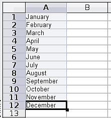
Using
a fill series
A more complex use of the Fill tool is to use a fill series. The default lists are for the full and abbreviated days of the week and the months of the year, but you can create your own lists as well.
To add a fill series to a spreadsheet, select the cells to fill, choose Edit → Fill → Series. In the Fill Series dialog (Figure 23), select AutoFill as the Series type, and enter as the Start value an item from any defined series. The selected cells then fill in the other items on the list sequentially, repeating from the top of the list when they reach the end of the list.
You can also use Edit → Fill → Series to create a one-time fill series for numbers by entering the start and end values and the increment. For example, if you entered start and end values of 1 and 7 with an increment of 2, you would get the sequence of 1, 3, 5, 7.
In all these cases, the Fill tool creates only a momentary connection between the cells. Once they are filled, the cells have no further connection with one another.
Defining a fill series
To define your own fill series:
Go to Tools → Options → LibreOffice Calc → Sort Lists. This dialog shows the previously-defined series in the Lists box on the left, and the contents of the highlighted list in the Entries box.
Click New. The Entries box is cleared.
Type the series for the new list in the Entries box (one entry per line). Click Add. The new list will now appear in the Lists box.
Click OK at the bottom of the dialog to save the new list.
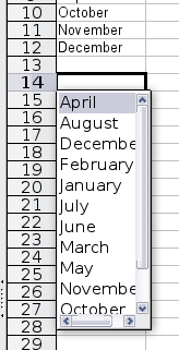
Selection lists are available only for text, and are limited to using only text that has already been entered in the same column.
To use a selection list, select a blank cell and press Ctrl+D. A drop-down list appears of any cell in the same column that either has at least one text character or whose format is defined as Text. Click on the entry you require.
Sharing content between sheets
You might want to enter the same information in the same cell on multiple sheets, for example to set up standard listings for a group of individuals or organizations. Instead of entering the list on each sheet individually, you can enter it in all the sheets at once. To do this, select all the sheets (Edit → Sheet → Select), then enter the information in the current one.
|
Caution
|
This technique overwrites any information that is already in the cells on the other sheets—without any warning. For this reason, when you are finished, be sure to deselect all the sheets except the one you want to edit. (Ctrl+click on a sheet tab to select or deselect the sheet.) |
When creating spreadsheets for other people to use, you may want to make sure they enter data that is valid or appropriate for the cell. You can also use validation in your own work as a guide to entering data that is either complex or rarely used.
Fill series and selection lists can handle some types of data, but they are limited to predefined information. To validate new data entered by a user, select a cell and use Data → Validity to define the type of contents that can be entered in that cell. For example, a cell might require a date or a whole number, with no alphabetic characters or decimal points; or a cell may not be left empty.
Depending on how validation is set up, the tool can also define the range of contents that can be entered and provide help messages that explain the content rules you have set up for the cell and what users should do when they enter invalid content. You can also set the cell to refuse invalid content, accept it with a warning, or start a macro when an error is entered.
See Chapter 2, Entering, Editing and Formatting Data, in the Calc Guide for more information.
Editing data is done in much the same way as entering data. The first step is to select the cell containing the data to be edited.
Data can be removed (deleted) from a cell in several ways.
Removing data only
The data alone can be removed from a cell without removing any of the formatting of the cell. Click in the cell to select it, and then press the Delete key.
Removing data and formatting
The data and the formatting can be removed from a cell at the same time. Press the Backspace key (or right-click and choose Delete Contents, or use Edit → Delete Contents) to open the Delete Contents dialog. From this dialog, the different aspects of the cell can be deleted. To delete everything in a cell (contents and format), check Delete all.
Replacing all the data in a cell
To remove data and insert new data, simply type over the old data. The new data will retain the original formatting.
Changing part of the data in a cell
Sometimes it is necessary to change the contents of cell without removing all of the contents, for example if the phrase “Sales in Qtr. 2” is in a cell and it needs to be changed to “Sales rose in Qtr. 2” It is often useful to do this without deleting the old cell contents first.
The process is the similar to the one described above, but you need to place the cursor inside the cell. You can do this in two ways.
Using the keyboard
After selecting the appropriate cell, press the F2 key and the cursor is placed at the end of the cell. Then use the keyboard arrow keys to move the cursor through the text in the cell.
Using the mouse
Using the mouse, either double-click on the appropriate cell (to select it and place the cursor in it for editing), or single-click to select the cell and then move the mouse pointer up to the input line and click into it to place the cursor for editing.
The data in Calc can be formatted in several ways. It can either be edited as part of a cell style so that it is automatically applied, or it can be applied manually to the cell. Some manual formatting can be applied using toolbar icons. For more control and extra options, select the appropriate cell or cells, right-click on it, and select Format Cells. All of the format options are discussed below.
|
Note |
All the settings discussed in this section can also be set as a part of the cell style. See Chapter 4, Using Styles and Templates in Calc, in the Calc Guide for more information. |
Formatting multiple lines of text
Multiple lines of text can be entered into a single cell using automatic wrapping or manual line breaks. Each method is useful for different situations.
Using automatic wrapping
To set text to wrap at the end of the cell, right-click on the cell and select Format Cells (or choose Format → Cells from the menu bar, or press Ctrl+1). On the Alignment tab (Figure 27), under Properties, select Wrap text automatically and click OK. The results are shown in Figure 28.
Using manual line breaks
To insert a manual line break while typing in a cell, press Ctrl+Enter. This method does not work with the cursor in the input line. When editing text, first double-click the cell, then single-click at the position where you want the line break.
When a manual line break is entered, the cell width does not change. Figure 29 shows the results of using two manual line breaks after the first line of text.
Shrinking text to fit the cell
The font size of the data in a cell can automatically adjust to fit in a cell. To do this, select the Shrink to fit cell size option in the Format Cells dialog (Figure 27). Figure 30 shows the results.
Several different number formats can be applied to cells by using icons on the Formatting toolbar. Select the cell, then click the relevant icon.
For more control or to select other number formats, use the Numbers tab (Figure 32) of the Format Cells dialog:
Apply any of the data types in the Category list to the data.
Control the number of decimal places and leading zeros.
Enter a custom format code.
The Language setting controls the local settings for the different formats such as the date order and the currency marker.
To quickly choose the font used in a cell, select the cell, then click the arrow next to the Font Name box on the Formatting toolbar and choose a font from the list.
|
Tip |
To choose whether to show the font names in their font or in plain text, go to Tools → Options → LibreOffice → View and select or deselect the Show preview of fonts option in the Font Lists section. For more information, see Chapter 2, Setting Up LibreOffice. |
To
choose the size of the font, click the arrow next to the Font Size
box on the Formatting toolbar. For other formatting, you can use the
Bold, Italic, or Underline icons.
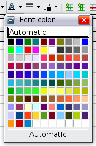
To choose a font color, click the arrow next to the Font Color icon to display the color palette. Click on the desired color.
(To define custom colors, use Tools → Options → LibreOffice → Colors. See Chapter 2.)
To specify the language of the cell (useful because it allows different languages to exist in the same document and be spell checked correctly), use the Font tab of the Format Cells dialog. Use the Font Effects tab to set other font characteristics. See Chapter 4, Using Styles and Templates in Calc, of the Calc Guide for more information.
To add a border to a cell (or group of selected cells), click on the Borders icon on the formatting toolbar, and select one of the border options displayed in the palette.
To quickly choose a line style and color for the borders of a cell, click the small arrows next to the Line Style and Line Color icons on the Formatting toolbar. In each case, a palette of choices is displayed.
For more controls, including the spacing between the cell borders and the text, use the Borders tab of the Format Cells dialog. There you can also define a shadow. See Chapter 4, Using Styles and Templates in Calc, of the Calc Guide for details.
|
Note |
The cell border properties apply to a cell, and can only be changed if you are editing that cell. For example, if cell C3 has a top border (which would be equivalent visually to a bottom border on C2), that border can only be removed by selecting C3. It cannot be removed in C2. |
Formatting the cell background
To quickly choose a background color for a cell, click the small arrow next to the Background Color icon on the Formatting toolbar. A palette of color choices, similar to the Font Color palette, is displayed.
(To define custom colors, use Tools → Options → LibreOffice → Colors. See Chapter 2 for more information.)
You can also use the Background tab of the Format Cells dialog. See Chapter 4, Using Styles and Templates in Calc, of the Calc Guide for details.
Autoformatting cells and sheets
You can use the AutoFormat feature to quickly apply a set of cell formats to a sheet or a selected cell range.
Select the cells, including the column and row headers, that you want to format.
Choose Format → AutoFormat.
|
Note |
The AutoFormat feature can only be applied if the selected set of cells consist of at least 3 columns and 3 rows and includes the column and row headers. |
To select which properties (number format, font, alignment, borders, pattern, autofit width and height) to include in an AutoFormat, click More. Select or deselect the required options.
Click OK.
If you do not see any change in color of the cell contents, choose View → Value Highlighting from the menu bar.
You can define a new AutoFormat that is available to all spreadsheets.
Format a sheet (in the style for the new AutoFormat).
Choose Edit → Select All.
Choose Format → AutoFormat. The Add button is now active.
Click Add.
In the Name box of the Add AutoFormat dialog, type a meaningful name for the new format.
Click OK to save. The new format is now available in the Format list in the AutoFormat dialog.
Formatting spreadsheets using themes
Calc comes with a predefined set of formatting themes that you can apply to your spreadsheets.
It is not possible to add themes to Calc, and they cannot be modified. However, you can modify their styles after you apply them to a spreadsheet.
To apply a theme to a spreadsheet:
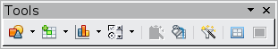
Click the Choose Themes icon in the Tools toolbar. If this toolbar is not visible, you can show it using View → Toolbars → Tools.
The Theme Selection dialog appears. This dialog lists the available themes for the whole spreadsheet.

In the Theme Selection dialog, select the theme that you want to apply to the spreadsheet.
As soon as you select a theme, some of the properties of the custom styles are applied to the open spreadsheet and are immediately visible.
Click OK. If you wish, you can now go to the Styles and Formatting window to modify specific styles. These modifications do not change the theme; they only change the appearance of this specific spreadsheet document.
You can set up cell formats to change depending on conditions that you specify. For example, in a table of numbers, you can show all the values above the average in green and all those below the average in red.
Conditional formatting depends upon the use of styles, and the AutoCalculate feature (Tools → Cell Contents → AutoCalculate) must be enabled. See Chapter 2, Entering, Editing, and Formatting Data, in the Calc Guide for details.
When elements are hidden, they are neither visible nor printed, but can still be selected for copying if you select the elements around them. For example, if column B is hidden, it is copied when you select columns A and C. When you need a hidden element again, you can reverse the process, and show the element.
To hide or show sheets, rows, and columns, use the options on the Format menu or the right-click (context) menu. For example, to hide a row, first select the row, and then choose Format → Row → Hide (or right-click and choose Hide).
To hide or show selected cells, choose Format → Cells from the menu bar (or right-click and choose Format Cells). On the Format Cells dialog, go to the Cell Protection tab.
If you are continually hiding and showing the same cells, you can simplify the process by creating outline groups, which add a set of controls for hiding and showing the cells in the group that are quick to use and always available.
If the contents of cells falls into a regular pattern, such as four cells followed by a total, then you can use Data → Group and Outline → AutoOutline to have Calc add outline controls based on the pattern. Otherwise, you can set outline groups manually by selecting the cells for grouping, then choosing Data → Group and Outline → Group. On the Group dialog, you can choose whether to group the selected cells by rows or columns.
When you close the dialog, the outline group controls are visible between either the row or column headers and the edges of the editing window. The controls resemble the tree-structure of a file-manager in appearance, and can be hidden by selecting Data → Outline → Hide Details. They are strictly for on screen use, and do not print.
The basic outline controls have plus or minus signs at the start of the group to show or hide hidden cells. However, if outline groups are nested, the controls have numbered buttons for hiding different levels.
If you no longer need a group, place the mouse cursor in any cell in it and select Data → Group and Outline → Ungroup. To remove all groups on a sheet, select Data → Group and Outline → Remove.
Filtering which cells are visible
A filter is a list of conditions that each entry has to meet in order to be displayed. You can set three types of filters from the Data → Filter sub-menu.
Automatic filters add a drop-down list to the top row of a column that contains commonly used filters. They are quick and convenient and are useful with text and with numbers, because the list includes every unique entry in the selected cells.
In addition to these unique entries, automatic filters include the option to display all entries, the ten highest numerical values, and all cells that are empty or not-empty, as well as a standard filter. The automatic filters are somewhat limited. In particular, they do not allow regular expressions, so you cannot use them to display cell contents that are similar, but not identical.
Standard filters are more complex than automatic filters. You can set as many as three conditions as a filter, combining them with the operators AND and OR. Standard filters are mostly useful for numbers, although a few of the conditional operators, such as = and < > can also be useful for text.
Other conditional operators for standard filters include options to display the largest or smallest values, or a percentage of them. Useful in themselves, standard filters take on added value when used to further refine automatic filters.
Advanced filters are structured similarly to standard filters. The differences are that advanced filters are not limited to three conditions, and their criteria are not entered in a dialog. Instead, advanced filters are entered in a blank area of a sheet, then referenced by the advanced filter tool to apply them.
Sorting arranges the visible cells on the sheet. In Calc, you can sort by up to three criteria, which are applied one after another. Sorts are handy when you are searching for a particular item, and become even more powerful after you have filtered data.
In addition, sorting is often useful when you add new information. When a list is long, it is usually easier to add new information at the bottom of the sheet, rather than adding rows in the proper places. After you have added information, you can then sort it to update the sheet.
Highlight the cells to be sorted, then select Data → Sort to open the Sort dialog (or click the Sort Ascending or Sort Descending toolbar buttons). Using the dialog, you can sort the selected cells using up to three columns, in either ascending (A-Z, 1-9) or descending (Z-A, 9-1) order.
On the Options tab of the Sort dialog, you can choose the following options:
Case sensitive
If two entries are otherwise identical, one with an upper case letter is placed before one with a lower case letter in the same position.
Range contains column labels
Does not include the column heading in the sort.
Include formats
A cell's formatting is moved with its contents. If formatting is used to distinguish different types of cells, then use this option.
Copy sort results to
Sets a spreadsheet address to which to copy the sort results. If a range is specified that does not have the necessary number of cells, then cells are added. If a range contains cells that already have content, then the sort fails.
Custom sort order
Select the box, then choose one of the sort orders defined in Tools → Options → Spreadsheet → Sort Lists from the drop-down list.
Direction
Sets whether rows or columns are sorted. The default is to sort by columns unless the selected cells are in a single column.
Printing from Calc is much the same as printing from other LibreOffice components (see Chapter 10), but some details are different, especially regarding preparation for printing.
Print ranges have several uses, including printing only a specific part of the data or printing selected rows or columns on every page. For more about using print ranges, see Chapter 6, Printing, Exporting, and E-mailing, in the Calc Guide.
To define a new print range or modify an existing print range:
Highlight the range of cells that comprise the print range.
Choose Format → Print Ranges → Define.
The page break lines display on the screen.
|
Tip |
You can check the print range by using File → Page Preview. LibreOffice will only display the cells in the print range. |
After defining a print range, you can add more cells to it. This allows multiple, separate areas of the same sheet to be printed, while not printing the whole sheet. After you have defined a print range:
Highlight the range of cells to be added to the print range.
Choose Format → Print Ranges → Add. This adds the extra cells to the print range.
The page break lines no longer display on the screen.
|
Note |
The additional print range will print as a separate page, even if both ranges are on the same sheet. |
Removing a print range
It may become necessary to remove a defined print range, for example if the whole sheet needs to be printed later.
Choose Format → Print Ranges → Remove. This removes all defined print ranges on the sheet. After the print range is removed, the default page break lines will appear on the screen.
Editing a print range
At any time, you can directly edit the print range, for example to remove or resize part of the print range. Choose Format → Print Ranges → Edit.
Selecting the page order, details, and scale
To select the page order, details, and scale to be printed:
Choose Format → Page from the main menu.
Select the Sheet tab.
Make your selections, and then click OK.
Page Order
When a sheet will print on more than one page, you can set the order in which pages print. This is especially useful in a large document; for example, controlling the print order can save time if you have to collate the document a certain way. The two available options are shown below.
|
Top to bottom, then right |
|
|
Left to right, then down |
|
Details
You can specify which details to print. These details include:
Row and column headers
Sheet grid—prints the borders of the cells as a grid
Comments—prints the comments defined in your spreadsheet on a separate page, along with the corresponding cell reference
Objects and graphics
Charts
Drawing objects
Formulas—prints the formulas contained in the cells, instead of the results
Zero Values—prints cells with a zero value
|
Note |
Remember that since the print detail options are a part of the page’s properties, they are also a part of the page style’s properties. Therefore, different page styles can be set up to quickly change the print properties of the sheets in the spreadsheet. |
Scale
Use the scale features to control the number of pages the data will print on. This can be useful if a large amount of data needs to be printed compactly or if you want the text enlarged to make it easier to read.
Reduce/Enlarge printout—scales the data in the printout either larger or smaller. For example if a sheet would normally print out as four pages (two high and two wide), a scaling of 50% would print as one page (both width and height are halved).
Fit print range(s) on number of pages—defines exactly how many pages the printout will take up. This option will only reduce a printout, it will not enlarge it. To enlarge a printout, the reduce/enlarge option must be used.
Fit print range(s) to width/height—defines how high and wide the printout will be, in pages.
Printing rows or columns on every page
If a sheet is printed on multiple pages, you can set up certain rows or columns to repeat on each printed page.
For example, if the top two rows of the sheet as well as column A need to be printed on all pages, do the following:
Choose Format → Print Ranges → Edit. On the Edit Print Ranges dialog, type the rows in the text entry box under Rows to repeat. For example, to repeat rows 1 and 2, type $1:$2. This automatically changes Rows to repeat from, - none - to - user defined -.
To repeat, type the columns in the text entry box under Columns to repeat. For example, to repeat column A, type $A. In the Columns to repeat list, - none - changes to - user defined -.
Click OK.
|
Note |
You do not need to select the entire range of the rows to be repeated; selecting one cell in each row works. |
While defining a print range can be a powerful tool, it may sometimes be necessary to manually adjust Calc’s printout. To do this, you can use a manual break. A manual break helps to ensure that your data prints properly. You can insert a horizontal page break above, or a vertical page break to the left of, the active cell.
Inserting a page break
To insert a page break:
Navigate to the cell where the page break will begin.
Select Insert → Manual Break.
Select Row Break or Column Break depending on your need.
The break is now set.
Row break
Selecting Row Break creates a page break above the selected cell. For example, if the active cell is H15, then the break is created between rows 14 and 15.
Column break
Selecting Column Break creates a page break to the left of the selected cell. For example, if the active cell is H15, then the break is created between columns G and H.
|
Tip |
To see page break lines more easily on screen, you can change their color. Choose Tools → Options → LibreOffice → Appearance and scroll down to the Spreadsheet section. |
Deleting a page break
To remove a page break:
Navigate to a cell that is next to the break you want to remove.
Select Edit → Delete Manual Break.
Select Row Break or Column Break depending on your need.
The break is now removed.
|
Note |
Multiple manual row and column breaks can exist on the same page. When you want to remove them, you have to remove each one individually. This may be confusing at times, because although there may be a column break set on the page, when you go to Edit → Manual Break, Column break may be grayed out. In order to remove the break, you have to be in the cell next to the break. For example, if you set the column break while you are in H15, you can not remove it if you are in cell D15. However, you can remove it from any cell in column H. |
Headers and footers are predefined pieces of text that are printed at the top or bottom of a sheet outside of the sheet area. Headers are set in the same way as footers.
Headers and footers are assigned to a page style. You can define more than one page style for a spreadsheet and assign different page styles to different sheets. For more about page styles, see Chapter 4, Using Styles and Templates, in the Calc Guide.
Setting a header or footer
To set a header or footer:
Navigate to the sheet that you want to set the header or footer for. Choose Format → Page.
On the Page Style dialog, select the Header (or Footer) tab. See Figure 38.
Select the Header on option.
From here you can also set the margins, the spacing, and height for the header or footer. You can check the AutoFit height box to automatically adjust the height of the header or footer.
Margin
Changing the size of the left or right margin adjusts how far the header or footer is from the side of the page.
Spacing
Spacing affects how far above or below the sheet the header or footer will print. So, if spacing is set to 1.00", then there will be 1 inch between the header or footer and the sheet.
Height
Height affects how big the header or footer will be.
Header or footer appearance
To change the appearance of the header or footer, click the More button in the header dialog. This opens the Border/Background dialog (Figure 39).
From this dialog you can set the background and border of the header or footer. For more information see Chapter 4, Using Styles and Templates, in the Calc Guide.
Setting the contents of the header or footer
The header or footer of a Calc spreadsheet has three columns for text. Each column can have different contents.
To set the contents of the header or footer, click the Edit button in the header or footer dialog shown in Figure 38 to display the dialog shown in Figure 40.
Areas
Each area in the header or footer is independent and can have different information in it.
Header
You can select from several preset choices in the Header drop-down list, or specify a custom header using the buttons below the area boxes. (To format a footer, the choices are the same.)
Custom header
Click in the area (Left, Center, Right) that you want to customize, then use the buttons to add elements or change text attributes.
![]() Opens the Text Attributes
dialog.
Opens the Text Attributes
dialog.
![]() Inserts the total number of
pages.
Inserts the total number of
pages.
![]() Inserts the File Name field.
Inserts the File Name field.
![]() Inserts the Date field.
Inserts the Date field.
![]() Inserts the Sheet Name field.
Inserts the Sheet Name field.
![]() Inserts the Time field.
Inserts the Time field.
![]() Inserts the current page number.
Inserts the current page number.