Calc Guide
Chapter
7
Using Formulas and Functions
This document is Copyright © 2005–2011 by its contributors as listed below. You may distribute it and/or modify it under the terms of either the GNU General Public License (http://www.gnu.org/licenses/gpl.html), version 3 or later, or the Creative Commons Attribution License (http://creativecommons.org/licenses/by/3.0/), version 3.0 or later.
All trademarks within this guide belong to their legitimate owners.
Contributors
Barbara Duprey
Hal Parker
Feedback
Please direct any comments or suggestions about this document to: documentation@libreoffice.org
Acknowledgments
This chapter is based on Chapter 7 of the OpenOffice.org 3.3 Calc Guide. The contributors to that chapter are:
Martin Fox Kirk Abbott Bruce
Byfield
Stigant Fyrwitful Barbara M. Tobias John Viestenz
Claire
Wood Jean Hollis Weber
Publication date and software version
Published 29 April 2011. Based on LibreOffice 3.3.
Some keystrokes and menu items are different on a Mac from those used in Windows and Linux. The table below gives some common substitutions for the instructions in this chapter. For a more detailed list, see the application Help.
|
Windows/Linux |
Mac equivalent |
Effect |
|
Tools → Options menu selection |
LibreOffice → Preferences |
Access setup options |
|
Right-click |
Control+click |
Open context menu |
|
Ctrl (Control) |
z (Command) |
Used with other keys |
|
F5 |
Shift+z+F5 |
Open the Navigator |
|
F11 |
z+T |
Open Styles & Formatting window |
Contents
Relative and absolute references 12
Calculations linking sheets 15
Understanding the structure of functions 20
Strategies for creating formulas and functions 24
Place a unique formula in each cell 25
Break formulas into parts and combine the parts 25
Use the Basic editor to create functions 26
#VALUE Non-existent value and #REF! Incorrect references 28
Basic arithmetic and statistic functions 30
In previous chapters, we have been entering one of two basic types of data into each cell: numbers and text. However, we will not always know what the contents should be. Often the contents of one cell depends on the contents of other cells. To handle this situation, we use a third type of data: the formula. Formulas are equations using numbers and variables to get a result. In a spreadsheet, the variables are cell locations that hold the data needed for the equation to be completed.
A function is a predefined calculation entered in a cell to help you analyze or manipulate data in a spreadsheet. All you have to do is add the arguments, and the calculation is automatically made for you. Functions help you create the formulas needed to get the results that you are looking for.
If you are setting up more than a simple one-worksheet system in Calc, it is worth planning ahead a little. Avoid the following traps:
Typing fixed values into formulas
Not including notes and comments describing what the system does, including what input is required and where the formulas come from (if not created from scratch)
Not incorporating a system of checking to verify that the formulas do what is intended
Many users set up long and complex formulas with fixed values typed directly into the formula.
For example, conversion from one currency to another requires knowledge of the current conversion rate. If you input a formula in cell C1 of =0.75*B1 (for example to calculate the value in Euros of the USD dollar amount in cell B1), you will have to edit the formula when the exchange rate changes from 0.75 to some other value. It is much easier to set up an input cell with the exchange rate and reference that cell in any formula needing the exchange rate. What-if type calculations also are simplified: what if the exchange rate varies from 0.75 to 0.70 or 0.80? No formula editing is needed and it is clear what rate is used in the calculations. Breaking complex formulas down into more manageable parts, described below, also helps to minimise errors and aid troubleshooting.
Lack of documentation is a very common failing. Many users prepare a simple worksheet which then develops into something much more complicated over time. Without documentation, the original purpose and methodology is often unclear and difficult to decipher. In this case it is usually easier to start again from the beginning, wasting the work done previously. If you insert comments in cells, and use labels and headings, a spreadsheet can be later modified by you or others and much time and effort will be saved.
Adding up columns of data or selections of cells from a worksheet often results in errors due to omitting cells, wrongly specifying a range, or double-counting cells. It is useful to institute checks in your spreadsheets. For example, set up a spreadsheet to calculate columns of figures, and use SUM to calculate the individual column totals. You can check the result by including (in a non-printing column) a set of row totals and adding these together. The two figures—row total and column total—must agree. If they do not, you have an error somewhere.
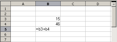
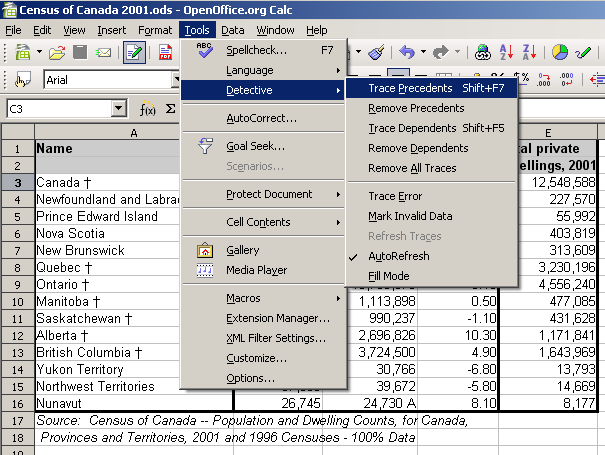
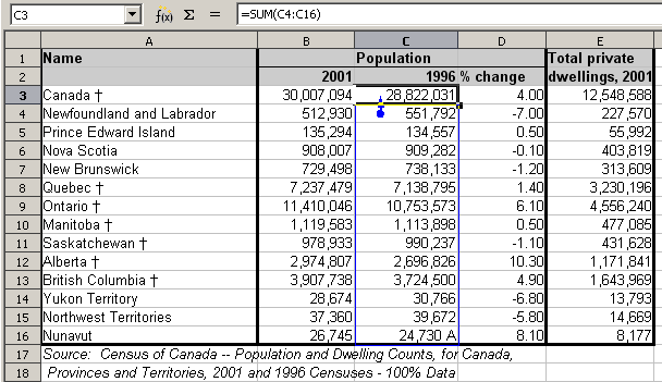
You can even set up a formula to calculate the difference between the two totals and report an error in case a non-zero result is returned (see Figure 1).
You can enter formulas in two ways, either directly into the cell itself, or at the input line. Either way, you need to start a formula with one of the following symbols: =, + or –. Starting with anything else causes the formula to be treated as if it were text.
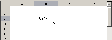
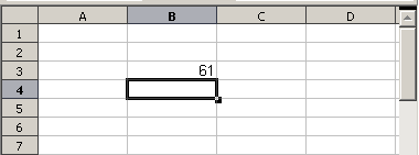
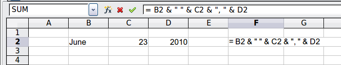
Each cell on the worksheet can be used as a data holder or a place for data calculations. Entering data is accomplished simply by typing in the cell and moving to the next cell or pressing Enter. With formulas, the equals sign indicates that the cell will be used for a calculation. A mathematical calculation like 15 + 46 can be accomplished as shown in Figure 2.
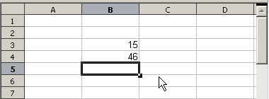
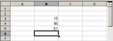
While the calculation on the left was accomplished in only one cell, the real power is shown on the right where the data is placed in cells and the calculation is performed using references back to the cells. In this case, cells B3 and B4 were the data holders, with B5 the cell where the calculation was performed. Notice that the formula was shown as =B3+B4. The plus sign indicates that the contents of cells B3 and B4 are to be added together and then have the result in the cell holding the formula. All formulas build upon this concept. Other ways of entering formulas are shown in Table 1.
These cell references allow formulas to use data from anywhere in the worksheet being worked on or from any other worksheet in the workbook that is opened. If the data needed was in different worksheets, they would be referenced by referring to the name of the worksheet, for example =SUM(Sheet2.B12+Sheet3.A11).
|
Note |
To enter the = symbol for a purpose other than creating a formula as described in this chapter, type an apostrophe or single quotation mark before the =. For example, in the entry '= means different things to different people, Calc treats everything after the single quotation mark—including the = sign—as text. |
|
Simple Calculation in 1 Cell |
Calculation by Reference |
|
|
|
|
|
|
|
|
|
Figure 2: A simple calculation
Table 1: Common ways to enter formulas
|
Formula |
Description |
|
=A1+10 |
Displays the contents of cell A1 plus 10. |
|
=A1*16% |
Displays 16% of the contents of A1. |
|
=A1*A2 |
Displays the result of the multiplication of A1 and A2. |
|
=ROUND(A1;1) |
Displays the contents of cell A1 rounded to one decimal place. |
|
=EFFECTIVE(5%;12) |
Calculates the effective interest for 5% annual nominal interest with 12 payments a year. |
|
=B8-SUM(B10:B14) |
Calculates B8 minus the sum of the cells B10 to B14. |
|
=SUM(B8;SUM(B10:B14)) |
Calculates the sum of cells B10 to B14 and adds the value to B8. |
|
=SUM(B1:B65536) |
Sums all numbers in column B. |
|
=AVERAGE(BloodSugar) |
Displays the average of a named range defined under the name BloodSugar. |
|
=IF(C31>140; "HIGH"; "OK") |
Displays the results of a conditional analysis of data from two sources. If the contents of C31 is greater than 140, then HIGH is displayed, otherwise OK is displayed. |
|
Note |
Users of Lotus 1-2-3®, Quattro Pro® and other spreadsheet software may be familiar with formulas that begin with +, -, =, (, @, ., $, or #. A mathematical formula would look like +D2+C2 or +2*3. Functions begin with the @ symbol such as @SUM(D2..D7), @COS(@DEGTORAD(30)) and @IRR(GUESS;CASHFLOWS). Ranges are identified such as A1..D3. |
Functions can be identified in Table 1 with a word, for example ROUND, followed by parentheses enclosing references or numbers.
It is also possible to establish ranges for inclusion by naming them using Insert → Names, for example BloodSugar representing a range such as B3:B10. Logical functions can also be performed as represented by the IF statement which results in a conditional response based upon the data in the identified cell, for example
=IF(A2>=0;"Positive";"Negative")
A value of 3 in cell A2 would return the result Positive, –9 the result Negative.
You can use the following operators in LibreOffice Calc: arithmetic, comparative, descriptive, text, and reference.
The addition, subtraction, multiplication and division operators return numerical results. The Negation and Percent operators identify a characteristic of the number found in the cell, for example -37. The example for Exponentiation illustrates how to enter a number that is being multiplied by itself a certain number of times, for example 23 = 2*2*2.
Table 2: Arithmetical operators
|
Operator |
Name |
Example |
|
+ (Plus) |
Addition |
=1+1 |
|
– (Minus) |
Subtraction |
=2–1 |
|
– (Minus) |
Negation |
–5 |
|
* (asterisk) |
Multiplication |
=2*2 |
|
/ (Slash) |
Division |
=10/5 |
|
% (Percent) |
Percent |
15% |
|
^ (Caret) |
Exponentiation |
2^3 |
Comparative operators are found in formulas that use the IF function and return either a true or false answer; for example, =IF(B6>G12; 127; 0) which, loosely translated, means if the contents of cell B6 are greater than the contents of cell G12, then return the number 127, otherwise return the number 0.
A direct answer of TRUE or FALSE can be obtained by entering a formula such as =B6>B12. If the numbers found in the referenced cells are accurately represented, the answer TRUE is returned, otherwise FALSE is returned.
Table 3: Comparative operators
|
Operator |
Name |
Example |
|
= (equal sign) |
Equal |
A1=B1 |
|
> (Greater than) |
Greater than |
A1>B1 |
|
< (Less than) |
Less than |
A1<B1 |
|
>= (Greater than or equal to) |
Greater than or equal to |
A1>=B1 |
|
<= (Less than or equal to) |
Less than or equal to |
A1<=B1 |
|
<> (Inequality) |
Inequality |
A1<>B1 |
If cell A1 contains the numerical value 4 and cell B1 the numerical value 5, the above examples would yield results of FALSE, FALSE, TRUE, FALSE, TRUE, and TRUE.
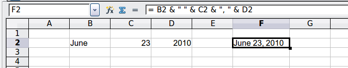
It is common for users to place text in spreadsheets. To provide for variability in what and how this type of data is displayed, text can be joined together in pieces coming from different places on the spreadsheet. Figure 3 shows an example.
|
|
|
|
|
|
|
Figure 3: Text concatenation |
In this example, specific pieces of the text were found in three different cells. To join these segments together, the formula also adds required spaces and punctuation enclosed within quotation marks, resulting in a formula of =B2 & " " & C2 & ", " & D2. The result is the concatenation into a date formatted in a particular sequence.
Calc has a CONCATENATE function which performs the same operation.
Taking this example further, if the result cell is defined as a name, then text concatenation is performed using this defined name. This process is demonstrated in Figures 4, 5, and 6 where the cell with the date is named “WizardDay” and subsequently used in a formula in another cell.
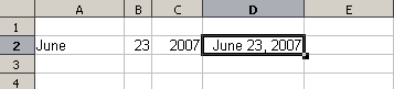
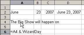
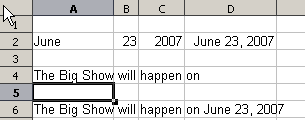
Figure 6: Defining Names on a worksheet
In its simplest form a reference refers to a single cell, but references can also refer to a rectangle or cuboid range or a reference in a list of references. To build such references you need reference operators.
An individual cell is identified by the column identifier (letter) located along the top of the columns and a row identifier (number) found along the left-hand side of the spreadsheet. On spreadsheets read from left to right, the upper left cell is A1.
Range operator
The range operator is written as colon. An expression using the range operator has the following syntax:
reference left : reference right
The range operator builds a reference to the smallest range including both the cells referenced with the left reference and the cells referenced with the right reference.
In the upper left corner of Figure 7 the reference A1:D12 is shown, corresponding to the cells included in the drag operation with the mouse to highlight the range.
Examples
|
A2:B4 |
Reference to a rectangle range with 6 cells, 2 column width × 3 row height. When you click on the reference in the formula in the input line, a border indicates the rectangle. |
|
(A2:B4):C9 |
Reference to a rectangle range with cell A2 top left and cell C9 bottom right. So the range contains 24 cells, 3 column width × 8 row height. This method of addressing extends the initial range from A2:B4 to A2:C9. |
|
Sheet1.A3:Sheet3.D4 |
Reference to a cuboid range with 24 cells, 4 column width × 2 row height × 3 sheets depth. |
When you enter B4:A2 or A4:B2 directly, then Calc will turn it to A2:B4. So the left top cell of the range is left of the colon and the bottom right cell is right of the colon. But if you name the cell B4 for example with _start and A2 with _end, you can use _start:_end without any error.
Calc can not reference a whole column of unspecified length using A:A or a whole row using 1:1 yet, as you might be familiar with in other spreadsheet programs.
Reference concatenation operator
The concatenation operator is written as a tilde. An expression using the concatenation operator has the following syntax:
reference left ~ reference right
The result of such an expression is a reference list, which is an ordered list of references. Some functions can take a reference list as an argument, SUM, MAX or INDEX for example.
The reference concatenation is sometimes called 'union'. But it is not the union of the two sets 'reference left' and 'reference right' as normally understood in set theory. COUNT(A1:C3~B2:D2) returns 12 (=9+3), but it has only 10 cells when considered as the union of the two sets of cells.
Notice that SUM(A1:C3;B2:D2) is different from SUM( A1:C3~B2:D2) although they give the same result. The first is a function call with 2 parameters, each of them is reference to a range. The second is a function call with 1 parameter, which is a reference list.
Intersection operator
The intersection operator is written as an exclamation mark. An expression using the intersection operator has the following syntax:
reference left ! reference right
If the references refer to single ranges, the result is a reference to a single range, containing all cells, which are both in the left reference and in the right reference.
If the references are reference lists, then each list item from the left is intersected with each one from the right and these results are concatenated to a reference list. The order is to first intersect the first item from the left with all items from the right, then intersect the second item from the left with all items from the right, and so on.
Examples
A2:B4 ! B3:D6
This results in a reference to the range B3:B4, because these cells are inside A2:B4 and inside B3:D4.
(A2:B4~B1:C2) ! (B2:C6~C1:D3)
First the intersections A2:B4!B2:C6, A2:B4!C1:D3, B1:C2!B2:C6 and B1:C2!C1:D3 are calculated. This results in B2:B4, empty, B2:C2, and C1:C2. Then these results are concatenated, dropping empty parts. So the final result is the reference list B2:B4 ~ B2:C2 ~ C1:C2.
You can use the intersection operator to refer a cell in a cross tabulation in an understandable way. If you have columns labeled 'Temperature' and 'Precipitation' and the rows labeled 'January', 'February', 'March', and so on, then the following expression
'February' ! !Temperature'
will reference to the cell containing the temperature in February.
The intersection operator (!) should have a higher precedence than the concatenation operator (~), but do not rely on precedence.
|
Tip |
Always put in parentheses the part that is to be calculated first. |
Relative and absolute references
References are the way that we refer to the location of a particular cell in Calc and can be either relative (to the current cell) or absolute (a fixed amount).
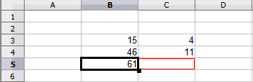
An example of a relative reference will illustrate the difference between a relative reference and absolute reference using the spreadsheet from Figure 8.
Type the numbers 4 and 11 into cells C3 and C4 respectively of that spreadsheet.
Copy the formula in cell B5 to cell C5. You can do this by using a simple copy and paste or click and drag B5 to C5 as shown below. The formula in B5 calculates the sum of values in the two cells B3 and B4.
Click in cell C5. The formula bar shows =C3+C4 rather than =B3+B4 and the value in C5 is 15, the sum of 4 and 11 which are the values in C3 and C4.
In cell B5 the references to cells B3 and B4 are relative references. This means that Calc interprets the formula in B5, applies it to the cells in the B column, and puts the result in the cell holding the formula. When you copied the formula to another cell, the same procedure was used to calculate the value to put in that cell. This time the formula in cell C5 referred to cells C3 and C4.

You can think of a relative address as a pair of offsets to the current cell. Cell B1 is 1 column to the left of Cell C5 and 4 rows above. The address could be written as R[-1]C[-4]. In fact earlier spreadsheets allowed this notation method to be used in formulas.
Whenever you copy this formula from cell B5 to another cell the result will always be the sum of the two numbers taken from the two cells one and two rows above the cell containing the formula.
Relative addressing is the default method of referring to addresses in Calc.
You may want to multiply a column of numbers by a fixed amount. A column of figures might show amounts in US Dollars. To convert these amounts to Euros it is necessary to multiply each dollar amount by the exchange rate. $US10.00 would be multiplied by 0.75 to convert to Euros, in this case Eur7.50. The following example shows how to input an exchange rate and use that rate to convert amounts in a column form USD to Euros.
Input the exchange rate Eur:USD (0.75) in cell D1. Enter amounts (in USD) into cells D2, D3 and D4, for example 10, 20, and 30.
In cell E2 type the formula =D2*D1. The result is 7.5, correctly shown.
Copy the formula in cell E2 to cell E3. The result is 200, clearly wrong! Calc has copied the formula using relative addressing - the formula in E3 is =D3*D2 and not what we want which is =D3*D1.
In cell E2 edit the formula to be =D2*$D$1. Copy it to cells E3 and E4. The results are now 15 and 22.5 which are correct.
The $ signs before the D and the 1 convert the reference to cell D1 from relative to absolute or fixed. If the formula is copied to another cell the second part will always show $D$1. The interpretation of this formula is “take the value in the cell one column to the left in the same row and multiply it by the value in cell D1”.
Cell references can be shown in four ways.
|
Reference |
Explanation |
|
D1 |
Relative, from cell E3 it is the cell one column to the left and two rows above |
|
$D$1 |
Absolute, from cell E3 it is the cell D1 |
|
$D1 |
Partially absolute, from cell E3 it is the cell in column D and two rows above |
|
D$1 |
Partially absolute, from cell E3 it is the cell one column to the left and in row 1 |
|
Tip |
To change references in formulas highlight the cell and press Shift-F4 to cycle through the four different types of references. This is of limited value in more complicated formulas, it is usually quicker to edit the formula by hand. |
Knowledge of the use of relative and absolute references is essential if you want to copy and paste formulas and to link spreadsheets.
Order of calculation refers to the sequence in which numerical operations are performed. Division and multiplication are performed before addition or subtraction. There is a common tendency to expect calculations to be made from left to right as the equation would be read in English. Calc evaluates the entire formula, then based upon programming precedence breaks the formula down executing multiplication and division operations before other operations. Therefore, when creating formulas you should test your formula to make sure that the correct result is being obtained. Following is an example of the order of calculation in operation.
Table 4 – Order of Calculation
|
Left To Right Calculation |
Ordered Calculation |
|
1+3*2+3 = 11 1+3=4, then 4 X 2 = 8, then 8 + 3 = 11 |
=1+3*2+3 result 10 3*2=6, then 1 + 6 + 3 = 10 |
|
Another possible intention could be: 1+3*2+3 = 20 |
The program resolves the multiplication of 3 X 2 before dealing with the numbers being added. |
If you intend for the result to be either of the two possible solutions on the left, the way to achieve these results would be to order the formula as:
|
((1+3) * 2)+3 = 11 |
(1+3) * (2+3) = 20 |
|
Note |
Use parentheses to group operations in the order you intend; for example, =B4+G12*C4/M12 might become =((B4+G12)*C4)/M12. |
Another powerful feature of Calc is the ability to link data through several worksheets. The naming of worksheets can be helpful to identify where specific data may be found. A name such as Payroll or Boise Sales is much more meaningful than Sheet1. The function named SHEET() returns the sheet number in the collection of spreadsheets. There are several worksheets in each book and they are numbered from the left: Sheet1, Sheet2, and so forth. If you drag the worksheets around to different locations among the tabs, the function returns the number referring to the current position of this worksheet.
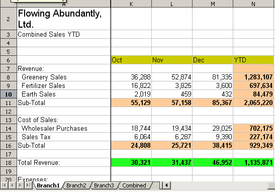
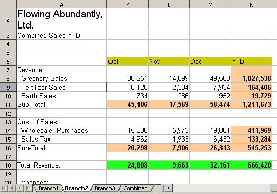
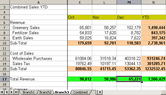
An example of calculations obtaining data from other work can be seen in a business setting where a business combines revenues and costs of each of its branch operations into a single combined worksheet.
|
|
Sheet containing data for Branch 1. |
|
|
Sheet containing data for Branch 2. |
|
|
Sheet containing data for Branch 3. |
|
|
Sheet containing combined data for all branches. |
|
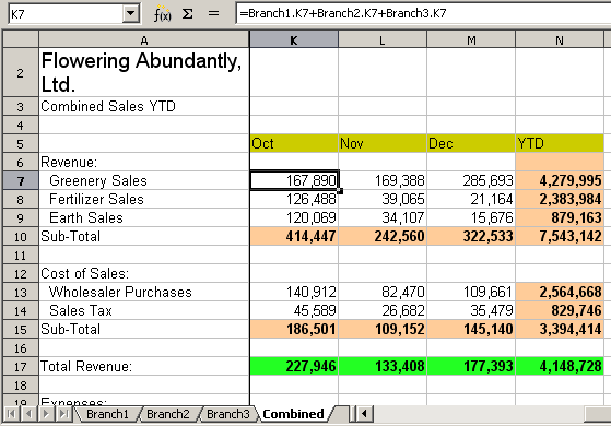
Figure 10: Combining data from several sheets into a single sheet |
|
The spreadsheets have been set up with identical structures. The easiest way to do this is to set up the first Branch spreadsheet, input data, format cells, and prepare the formulas for the various sums of rows and columns.
On the worksheet tab, right-click and select Rename Sheet. Type Branch1. Right-click on the tab again and select Move/Copy Sheet.
In the Move/Copy Sheet dialog, select the Copy option and select Sheet 2 in the area Insert before. Click OK, right-click on the tab of the sheet Branch1_2 and rename it to Branch2. Repeat to produce the Branch3 and Combined worksheets.

Enter the data for Branch 2 and Branch 3 into the respective sheets. Each sheet stands alone and reports the results for the individual branches.
In the Combined worksheet, click on cell K7. Type =, click on the tab Branch1, click on cell K7, press +, repeat for sheets Branch2 and Branch3 and press Enter. You now have a formula in cell K1 which adds the revenue from Greenery Sales for the 3 Branches.
Copy the formula, highlight the range K7..N17, click Edit → Paste Special, uncheck the Paste all and Formats boxes in the Selection area of the dialog box and click OK. You will see the following message:
Click Yes. You have now copied the formulas into each cell while maintaining the format you set up in the original worksheet. Of course, in this example you would have to tidy the worksheet up by removing the zeros in the non-formatted rows.

|
Note |
LibreOffice default is to paste all the attributes of the original cell(s) - formats, notes, objects, text strings and numbers. |
The Function Wizard can also be used to accomplish the linking. Use of this Wizard is described in detail in the section on Functions.
Calc includes over 350 functions to help you analyze and reference data. Many of these functions are for use with numbers, but many others are used with dates and times, or even text. A function may be as simple as adding two numbers together, or finding the average of a list of numbers. Alternatively, it may be as complex as calculating the standard deviation of a sample, or a hyperbolic tangent of a number.
Typically, the name of a function is an abbreviated description of what the function does. For instance, the FV function gives the future value of an investment, while BIN2HEX converts a binary number to a hexadecimal number. By tradition, functions are entered entirely in upper case letters, although Calc will read them correctly if they are in lower or mixed case, too.
A few basic functions are somewhat similar to operators. Examples:
|
+ |
This operator adds two numbers together for a result. SUM() on the other hand adds groups of contiguous ranges of numbers together. |
|
* |
This operator multiplies two numbers together for a result. PRODUCT() does the same for multiplying that SUM() does for adding. |
Each function has a number of arguments used in the calculations. These arguments may or may not have their own name. Your task is to enter the arguments needed to run the function. In some cases, the arguments have predefined choices, and you may need to refer to the online help or Appendix B (Description of Functions) in this book to understand them. More often, however, an argument is a value that you enter manually, or one already entered in a cell or range of cells on the spreadsheet. In Calc, you can enter values from other cells by typing in their name or range, or—unlike the case in some spreadsheets—by selecting cells with the mouse. If the values in the cells change, then the result of the function is automatically updated.
For compatibility, functions and their arguments in Calc have almost identical names to their counterparts in Microsoft Excel. However, both Excel and Calc have functions that the other lacks. Occasionally, functions with the same names in Calc and Excel have different arguments, or slightly different names for the same argument—neither of which can be imported to the other. However, the majority of functions can be used in both Calc and Excel without any change.
Understanding the structure of functions
All functions have a similar structure. If you use the right tool for entering a function, you can escape learning this structure, but it is still worth knowing for troubleshooting.
To give a typical example, the structure of a function to find cells that match entered search criteria is:
= DCOUNT (Database;Database field;Search_criteria)
Since a function cannot exist on its own, it must always be part of a formula. Consequently, even if the function represents the entire formula, there must be an = sign at the start of the formula. Regardless of where in the formula a function is, the function will start with its name, such as DCOUNT in the example above. After the name of the function comes its arguments. All arguments are required, unless specifically listed as optional.
Arguments are added within the parentheses and are separated by semicolons, with no space between the arguments and the semicolons.
|
Note |
LibreOffice uses the semicolon as an argument list separator, unlike Excel which uses a comma. This is a common mistake made by users accustomed to entering Excel formulas. |
Many arguments are a number. A Calc function can take up to thirty numbers as an argument. That may not sound like much at first. However, when you realize that the number can be not only a number or a single cell, but also an array or range of cells that contain several or even hundreds of cells, then the apparent limitation vanishes.
Depending on the nature of the function, arguments may be entered as follows:
|
"text data" |
The quotes indicate text or string data is being entered. |
|
9 |
The number nine is being entered as a number. |
|
"9" |
The number nine is being entered as text |
|
A1 |
The address for whatever is in Cell A1 is being entered |
Functions can also be used as arguments within other functions. These are called nested functions.
=SUM(2;PRODUCT(5;7))
To get an idea of what nested functions can do, imagine that you are designing a self-directed learning module. During the module, students do three quizzes, and enter the results in cells A1, A2, and A3. In A4, you can create a nested formula that begins by averaging the results of the quizzes with the formula =AVERAGE(A1:A3). The formula then uses the IF function to give the student feedback that depends upon the average grade on the quizzes. The entire formula would read:
=IF(AVERAGE(A1:A3) >85; "Congratulations! You are ready to advance to the next module"; "Failed. Please review the material again. If necessary, contact your instructor for help")
Depending on the average, the student would receive the message for either congratulations or failure.
Notice that the nested formula for the average does not require its own equal sign. The one at the start of the equation is enough for both formulas.
If you are new to spreadsheets, the best way to think of functions is as a scripting language. We've used simple examples to explain the concept more clearly, but, through nesting of functions, a Calc formula can quickly become complex.
|
Note |
Calc keeps the syntax of a formula displayed in a tool tip next to the cell as a handy memory aid as you type. |
A more reliable method is to use the Function List (Figure 15).
Available from the Insert menu, the Function List automatically docks as a pane on the right side of the Calc editing window. If you wish, you can Control+double-click on a blank space at the top of the pane to undock this pane and make it a floating window.
The Function List includes a brief description of each function and its arguments; highlight the function and look at the bottom of the pane to see the description. If necessary, hover the cursor over the division between the list and the description; when the cursor becomes a two-headed arrow, drag it upwards to increase the space for the description. Double-click on a function’s name to add it to the current cell, together with placeholders for each of the function’s arguments.
Clicking on the bar where the 5 dots and arrows are shown (shown by the ellipse in Figure 15) will hide the list on the right hand side of the screen. Clicking this area again will show the list, making it easy to keep the list available for easy reference.
Using the Function List is almost as fast as manual entry, and has the advantage of not requiring that you memorize a formula that you want to use. In theory, it should also be less error-prone. In practice, though, some users may fumble when replacing the placeholders with values. Another feature is the ability to display the last formulas used.
The most commonly used input method is the Function Wizard (Figure 17). To open the Function Wizard, choose Insert → Function, or click the fx button on the Function tool bar, or press Ctrl+F2. Once open, the Function Wizard provides the same help features as the Function List, but adds fields in which you can see the result of a completed function, as well as the result of any larger formula of which it is part.
Select a category of functions to shorten the list, then scroll down through the named functions and select the required one. When you select a function its description appears on the right-hand side of the dialog. Double-click on the required function.
The
Wizard now displays an area to the right where you can enter data
manually in text boxes or click the Shrink
button
![]() to
shrink the wizard so you can select cells from the worksheet.
to
shrink the wizard so you can select cells from the worksheet.

To select cells, either click directly upon the cell or hold down the left mouse button and drag to select the required area.
When the area has been selected, click the Shrink button again to return to the wizard.
If multiple arguments are needed select the next text box below the first and repeat the selection process for the next cell or range of cells. Repeat this process as often as required. The Wizard will accept up to 30 ranges or arguments in the SUM function.
Click OK to accept the function and add it to the cell and get the result.
You can also select the Structure tab (Figure 18) to see a tree view of the parts of the formula. The main advantage over the Function List is that each argument is entered in its own field, making it easier to manage. The price of this reliability is slower input, but this is often a small price to pay, since precision is generally more important than speed when creating a spreadsheet.
After you enter a function on the Input line, press the Enter key or click the Accept button on the Function toolbar to add the function to the cell and get its result.
If you see the formula in the cell instead of the result, then Formulas are selected for display in Tools → Options → LibreOffice Calc → View → Display. Deselect Formulas, and the result will display. However, you can still see the formula in the Input line.
Strategies for creating formulas and functions
Formulas that do more than a simple calculation or summation of rows or columns of values usually take a number of arguments. For example, the classic equation of motion s = s0+ vt - ½at2 calculates the position of a body knowing its original position, its final velocity, its acceleration, and the time taken to move from the initial state to the final state.
For ease of presentation, it is good practice to set up a spreadsheet in a manner similar to that shown in Figure 20. In this example, the individual variables are input into cells on the sheet and no editing of the formula (in cell B9) is required.
You can take several broad approaches when creating a formula. In deciding which approach to take, consider how many other people will need to use the worksheets, the life of the worksheets, and the variations that could be encountered in use of the formula.
If people other than yourself will use the spreadsheet, make sure that it is easy to see what input is required and where. Explanation of the purpose of the spreadsheet, basis of calculation, input required and output(s) generated are often placed on the first worksheet.
A spreadsheet that you build today, with many complicated formulas, may not be quite so obvious in its function and operation in 6 or 12 months time. Use comments and notes liberally to document your work.
You might be aware that you cannot use negative values or zero values for a particular argument, but if someone else inputs such a value will your formula be robust or simply return a standard (and often not too helpful) Err: message? It is a good idea to trap errors using some form of logic statements or with conditional formatting.
Place a unique formula in each cell
The most basic strategy is to view whatever formulas are needed as simple and with a limited useful life. The strategy is then to place a unique formula in each appropriate cell. This can be recommended only for very simple or “throw away” (single use) spreadsheets.
Break formulas into parts and combine the parts
The second strategy is similar to the first, but instead you break down longer formulas into smaller parts and then combine the parts into the whole. Many examples of this type exist in complex scientific and engineering calculations where interim results are used in a number of places in the worksheet. The result of calculating the flow velocity of water in a pipe may be used in estimating losses due to friction, whether the pipe is flowing full or partially empty, and in optimizing the diameter for the given flow regime.
In all cases you should adopt the basic principles of formula creation described previously.
Use the Basic editor to create functions
A third strategy is to use the Basic editor and create your own functions and macros. This approach would be used where the result would greatly simplify the use of the spreadsheet by the end user and keep the formulas simple with a better chance of avoiding errors. This approach also can make the maintenance easier by having corrections or updates kept in one central location. The use of macros is described in Chapter 12 of this book and is a specialized topic in itself. The danger of overusing macros and custom functions is that the principles upon which the spreadsheet is based become much more difficult to see by a user other than the original author (and sometimes even by the author!).
It is common to find situations where errors are displayed. Even with all the tools available in Calc to help you to enter formulas, making mistakes is easy. Many people find inputting numbers difficult and many may make a mistake about the kind of entry that a function's argument needs. In addition to correcting errors, you may want to find the cells used in a formula to change their values or to check the answer.
Calc provides three tools for investigating formulas and the cells that they reference: error messages, color coding, and the Detective.
The most basic tool is error messages. Error messages display in a formula’s cell or in the Function Wizard instead of the result.
An error message for a formula is usually a three-digit number from 501 to 527, or sometimes an unhelpful piece of text such as NAME?, REF, or VALUE. The error number appears in the cell, and a brief explanation of the error on the right side of the status bar.
Most error messages indicate a problem with how the formula was input, although several indicate that you have run up against a limitation of either Calc or its current settings.
Error messages are not user-friendly, and may intimidate new users. However, they are valuable clues to correcting mistakes. You can find detailed explanations of them in the help, by searching for Error codes in LibreOffice Calc. A few of the most common are shown in the following table.
|
NAME? (525) |
No valid reference exists for the argument. |
|
REF (525) |
The column, row, or sheet for the referenced cell is missing. |
|
VALUE (519) |
The value for one of the arguments is not the type that the argument requires. The value may be entered incorrectly; for example, double-quotation marks may be missing around the value. At other times, a cell or range used may have the wrong format, such as text instead of numbers. |
|
509 |
An operator such as an equals sign is missing from the formula. |
|
510 |
An argument is missing from the formula. |
|
502 |
The column, row, or sheet for the referenced cell is missing. |
This error is the result of dividing a number by either the number zero (0) or a blank cell. There is an easy way to avoid this type of problem. When you have a zero or blank cell displayed, use a conditional function. Figure 21 depicts division of column B by column C yielding 2 errors arising from a zero and a blank cell showing in column C.
It is very common to find an error such as this arising from a situation where data was not reported or reported incorrectly. When such an occurrence is possible, an IF function can be used to display the data correctly. The formula =IF(C3>0, B3/C3, "No Report") can be entered. The formula is then copied over the remainder of Column D. The meaning of this formula roughly would be: “If C3 is greater than 0, then compute B3 divided by C3, otherwise enter ‘No Report’”.
It is also possible for the last parameter to use double quotes for a blank to be entered, or a different formula with a standardized number being substituted for the lower number. An example of this might be to use the nursing staff in the unit.

#VALUE Non-existent value and #REF! Incorrect references
The non-existent value error is also very common. The most common appearance of this error arises when a user copies a formula over a selected area. When copying, it is typical for the program to increment the represented cells. If you were copying downward from cell B3 the program would automatically substitute the cell B4 into the next lower cell and so on until the end of the copying process. If that next cell contains text or a value that is inappropriate for the formula, then this error may result. The difficulty usually occurs when one or more of the parameters in the formula need to be fixed.
|
Note |
To avoid the #VALUE and #REF! errors, give the cell B3 a name such as TotalExpenses. In that way, the program will carry that name to each succeeding formula being copied and remove the need to use the $ to anchor the reference to the TotalExpenses cell. |
Another useful tool when reviewing a formula is the color coding for input. When you select a formula that has already been entered, the cells or ranges used for each argument in the formula are outlined in color.
Calc uses eight colors for outlining referenced cells, starting with blue for the first cell, and continuing with red, magenta, green, dark blue, brown, purple and yellow before cycling through the sequence again.
In a long or complicated spreadsheet, color coding becomes less useful. In these cases, consider using the the submenu under Tools → Detective. The Detective is a tool for checking which cells are used as arguments by a formula (precedents) and which other formulas it is nested in (dependents), and tracking errors. It can also be used for tracing errors, marking invalid data (that is, information in cells that is not in the proper format for a function’s argument), or even for removing precedents and dependents.
To use the Detective, select a cell with a formula, then start the Detective. On the spreadsheet, you will see lines ending in circles to indicate precedents, and lines ending in arrows for dependents. The lines show the flow of information.
Use the Detective to assist in following the precedents referred to in a formula in a cell. By tracing these precedents, you frequently can find the source of the errors. Place the cursor in the cell in question and then choose Tools → Detective → Trace Precedents from the menu bar or press Shift+F7. Figure 23 shows a simple example of tracing precedents.
|
Cursor placed in cell |
|
Figure 23: Tracing precedents using the Detective |
|
a) Initiate trace by clicking Trace Precedents |
|
b) Source area highlighted in Blue, with arrow pointing to the calculation cell |
(continued): Tracing precedents using the Detective
We are concerned that the number shown in Cell C3 is incorrectly stated. The cause can be seen in the highlighted cells. In this case cell C16 contains both numeric data as well as letters. Removing the letters resolves the problem in the calculation.
In other cases we must trace the error. Use the Trace Error function, found under Tools → Detective → Trace Error, to find the cells that cause the error.
For novices, functions are one of the most intimidating features of LibreOffice's Calc. New users quickly learn that functions are an important feature of spreadsheets, but there are almost four hundred, and many require input that assumes specialized knowledge. Fortunately, Calc includes dozens of functions that anyone can use.
Basic arithmetic and statistic functions
The most basic functions create formulas for basic arithmetic or for evaluating numbers in a range of cells.
The simple arithmetic functions are addition, subtraction, multiplication, and division.
Except for subtraction, each of these operations has its own function:
SUM for addition
PRODUCT for multiplication
QUOTIENT for division
Traditionally, subtraction does not have a function.
SUM, PRODUCT, and QUOTIENT are useful for entering ranges of cells in the same way as any other function, with arguments in brackets after the function name.
However, for basic equations, many users prefer the time-honored computer symbols for these operations, using the plus sign (+) for addition, the hyphen (–) for subtraction, the asterisk (*) for multiplication and the forward slash (/) for division. These symbols are quick to enter without requiring your hands to stray from the keyboard.
A similar choice is also available if you want to raise a number by the power of another. Instead of entering =POWER(A1;2), you can enter =A1^2.
Moreover, they have the advantage that you enter formulas with them in an order that more closely approximates human readable format than the spreadsheet-readable format used by the equivalent function. For instance, instead of entering =SUM (A1:A2), or possibly =SUM (A1;A2), you enter =A1+A2. This almost-human readable format is especially useful for compound operations, where writing =A1*(A2+A3) is briefer and easier to read than =PRODUCT(A1;SUM(A2:A3)).
The main disadvantage of using arithmetical operators is that you cannot directly use a range of cells. In other words, to enter the equivalent of =SUM (A1:A3), you would need to type =A1+A2+A3.
Otherwise, whether you use a function or an operator is largely up to you—except, of course, when you are subtracting. However, if you use spreadsheets regularly in a group setting such as a class or an office, you might want to standardize on an entry format so that everyone who handles a spreadsheet becomes accustomed to a standard input.
Another common use for spreadsheet functions is to pull useful information out of a list, such as a series of test scores in a class, or a summary of earnings per quarter for a company.
You can, of course, scan a list of figures if you want basic information such as the highest or lowest entry or the average. The only trouble is, the longer the list, the more time you waste and the more likely you are to miss what you’re looking for. Instead, it is usually quicker and more efficient to enter a function. Such reasons explain the existence of a function like COUNT, which does no more than give the total number of entries in the designated cell range.
Similarly, to find the highest or lowest entry, you can use MIN or MAX. For each of these formulas, all arguments are either a range of cells, or a series of cells entered individually.
Each also has a related function, MINA or MAXA, which performs the same function, but treats a cell formatted for text as having a value of 0 (The same treatment of text occurs in any variation of another function that adds an "A" to the end). Either function gives the same result, and could be useful if you used a text notation to indicate, for example, if any student were absent when a test was written, and you wanted to check whether you needed to schedule a makeup exam.
For more flexibility in similar operations, you could use LARGE or SMALL, both of which add a specialized argument of rank. If the rank is 1 used with LARGE, you get the same result as you would with MAX. However, if the rank is 2, then the result is the second largest result. Similarly, a rank of 2 used with SMALL gives you the second smallest number. Both LARGE and SMALL are handy as a permanent control, since, by changing the rank argument, you can quickly scan multiple results.
You would need to be an expert to want to find the Poisson Distribution of a sample, or to find the skew or negative binomial of a distribution (and, if you are, you will find functions in Calc for such things). However, for the rest of us, there are simpler statistical functions that you can quickly learn to use.
In particular, if you need an average, you have a number to choose from. You can find the arithmetical means—that is, the result when you add all entries in a list then divided by the number of entries by enter a range of numbers when using AVERAGE, or AVERAGE A to include text entries and to give them a value of zero.
In addition, you can get other information about the data set:
MEDIAN: The entry that is exactly half way between the highest and lowest number in a list.
MODE: The most common entry in a list of numbers.
QUARTILE:The entry at a set position in the array of numbers. Besides the cell range, you enter the type of Quartile: 0 for the lowest entry, 1 for the value of 25%, 2 for the value of 50%, 3 for 75%, and 4 for the highest entry. Note that the result for types 1 through 3 may not represent an actual item entered.
RANK: The position of a given entry in the entire list, measured either from top to bottom or bottom to top. You need to enter the cell address for the entry, the range of entries, and the type of rank (0 for the rank from the highest, or 1 for the rank from the bottom.
Some of these functions overlap; for example, MIN and MAX are both covered by QUARTILE. In other cases, a custom sort or filter might give much the same result. Which you use depends on your temperament and your needs. Some might prefer to use MIN and MAX because they are easy to remember, while others might prefer QUARTILE because it is more versatile.
In some cases, you may be able to get similar results to some of these functions by setting up a filter or a custom sort. However, in general, functions are more easily adjusted than filters or sorts, and provide a wide range of possibilities.
At times, you may just want to enter one or more formulas temporarily in a convenient blank cell, and delete it once you have finished. However, if you find yourself using the same functions constantly, you should consider creating a template and including space for all the functions you use, with the cell to their left used as a label for them. Once you have created the template, you can easily update each formula as entries change, either automatically and on-the-fly or pressing the F9 key to update all selected cells.
No matter how you use these functions, you will probably find them simple to use and adaptable for many purposes. By the time you have mastered this handful, you will be ready to try more complex functions.
For statistical and mathematical purposes, Calc includes a variety of ways to round off numbers. If you’re a programmer, you may also be familiar with some of these methods. However, you don’t need to be a specialist to find some of these methods useful. You may want to round off for billing purposes, or because decimal places don’t translate well into the physical world—for instance, if the parts you need come in packages of 100, then the fact you only need 66 is irrelevant to you; you need to round up for ordering. By learning the options for rounding up or down, you can make your spreadsheets more immediately useful.
When you use a rounding function, you have two choices about how to set up your formulas. If you choose, you can nest a calculation within one of the rounding functions. For instance, the formula =ROUND((SUM(A1;A2)) adds the figures in cells A1 and A2, then rounds them off to the nearest whole number. However, even though you don’t need to work with exact figures every day, you may still want to refer to them occasionally. If that is the case, then you are probably better off separating the two functions, placing =SUM(A1;A2) in cell A3, and =ROUND (A3) in A4, and clearly labelling each function.
The most basic function for rounding numbers in Calc is ROUND. This function will round off a number according to the usual rules of symmetric arithmetic rounding: a decimal place of .4 or less gets rounded down, while one of .5 or more gets rounded up. However, at times, you may not want to follow these rules. For instance, if you are one of those contractors who bills a full hour for any fraction of an hour you work, you would want to always round up so you didn’t lose any money. Conversely, you might choose to round down to give a slight discount to a long-established customer. In these cases, you might prefer to use ROUNDUP or ROUNDDOWN, which, as their names suggest, round a number to the nearest integer above or below it.
All three of these functions require the single argument of number—the cell or number to be rounded. Used with only this argument, all three functions round to the nearest whole number, so that 46.5 would round to 47 with ROUND or ROUNDUP and 46 with ROUNDDOWN. However, if you use the optional count argument, you can specify the number of decimal places to include. For instance, if number was set to 1, then 48.65 would round to 48.7 with ROUND or ROUNDUP and to 48.6 with ROUNDDOWN.
As an alternative to ROUNDDOWN when working with decimals, you can use TRUNC (short for truncate). It takes exactly the same arguments as ROUNDDOWN, so which function you use is a matter of choice. If you aren't working with decimals, you might choose to use INT (short for integer), which takes only the number argument.
Another option is the ODD and EVEN pair of functions. ODD rounds up to the nearest odd number if what is entered in the number argument is a positive number, and rounds down if it is a negative number, while EVEN does the same for an even number.
Options are the CEILING and FLOOR functions. As you can guess from the names, CEILING rounds up and FLOOR rounds down. For both functions, the number that they round to is determined by the closest multiple of the number that you enter as the significance argument. For instance, if your business insurance is billed by the work week, the fact that you were only open three days one week would be irrelevant to your costs; you would still be charged for an entire week, and therefore might want to use CEILING in your monthly expenses.
Conversely, if you are building customized computers and completed 4.5 in a day, your client would only be interested in the number ready to ship, so you might use FLOOR in a report of your progress. If cell E1 contains the value 46.7, =CEILING(E1;7) will return the value 49.
Besides number and significance, both CEILING and FLOOR include an optional argument called mode, which takes a value of 0 or 1. If mode is set to 0, and both the number and the significance are negative numbers, then the result of either function is rounded up; if it is set to 1, and both the number and the significance are negative numbers, then the results are rounded down. In other words, if the number is -11 and the significance is -5, then the result is -10 when the mode is set to 0, but -15 when set to 1.
However, if you are exchanging spreadsheets between Calc and MS Excel, remember that the mode argument is not supported by Excel. If you want the answers to be consistent between the two spreadsheets, set the mode in Calc to -1.
A function somewhat similar to CEILING and FLOOR is MROUND. Like CEILING AND FLOOR, MROUND requires two arguments, although, somewhat confusingly, the second one is called multiple rather than significance, even though the two are identical. The difference between MROUND and CEILING and FLOOR is that MROUND rounds up or down using symmetric arithmetic rounding. For example, if the number is 77 and the multiple is 5, then MROUND gives a result of 75. However, if the multiple is changed to 7, then MROUND's result becomes 77.
Once you become familiar with Calc’s long, undifferentiated list of functions, you can start to decide which is most useful for your purposes.
However, one last point is worth mentioning: If you are working with more than two decimal places, don't be surprised if you don’t see the same number of decimal places on the spreadsheet as you do on the function wizard. If you don’t, the reason is that Tools → Options → LibreOffice Calc → Calculate → Decimal Places defaults to 2. Change the number of decimal places, and, if necessary, uncheck the Precision as shown box on the same page, and the spreadsheet will display as expected.
Using regular expressions in functions
A number of functions in Calc allow the use of regular expressions: SUMIF, COUNTIF, MATCH, SEARCH, LOOKUP, HLOOKUP, VLOOKUP, DCOUNT, DCOUNTA, DSUM, DPRODUCT, DMAX, DMIN, DAVERAGE, DSTDEV, DSTDEVP, DVAR, DVARP, DGET.
Whether or not regular expressions are used is selected on the Tools → Options → LibreOffice Calc → Calculate dialog.
For example =COUNTIF(A1:A6;"r.d") with Enable regular expressions in formulas selected will count cells in A1:A6 which contain red and ROD.
Additionally if Search criteria = and <> must apply to whole cells is not selected, then Fred, bride, and Ridge will also be counted. If that setting is selected, then it can be overcome by wrapping the expression thus: =COUNTIF(A1:A6;".*r.d.*").
Regular expression searches within functions are always case insensitive, irrespective of the setting of the Case sensitive checkbox on the dialog in Figure 24—so red and ROD will always be matched in the above example. This case-insensitivity also applies to the regular expression structures ([:lower:]) and ([:upper:]), which match characters irrespective of case.
Regular expressions will not work in simple comparisons. For example: A1="r.d" will always return FALSE if A1 contains red, even if regular expressions are enabled. It will only return TRUE if A1 contains r.d (r then a dot then d). If you wish to test using regular expressions, try the COUNTIF function: COUNTIF(A1; "r.d") will return 1 or 0, interpreted as TRUE or FALSE in formulas like =IF(COUNTIF(A1; "r.d");"hooray"; "boo").
Activating the Enable regular expressions in formulas option means all the above functions will require any regular expression special characters (such as parentheses) used in strings within formulas, to be preceded by a backslash, despite not being part of a regular expression. These backslashes will need to be removed if the setting is later deactivated.
As is common with other spreadsheet programs, LibreOffice Calc can be enhanced by user-defined functions or add-ins. Setting up user-defined functions can be done either by using the Basic IDE or by writing separate add-ins or extensions.
The basics of writing and running macros is covered in Chapter 12, Calc Macros. Macros can be linked to menus or toolbars for ease of operation or stored in template modules to make the functions available in other documents.
Calc Add-ins are specialized office extensions which can extend the functionality of LibreOffice with new built-in Calc functions. Writing Add-ins requires knowledge of the C++ language, the LibreOffice SDK, and is for experienced programmers. A number of extensions for Calc have been written and these can be found on the extensions site at http://extensions.libreoffice.org/. Refer to Chapter 14, Setting up and Customizing Calc, for more details.