Calc Guide

Chapter 9
Data Analysis

Using Scenarios, Goal Seek, Solver, others

Introduction

Once you are familiar with functions and formulas, the next step is to learn how to use Calc's automated processes to quickly perform useful analysis of your data.

Calc includes several tools to help you manipulate the information in your spreadsheets, ranging from features for copying and reusing data, to creating subtotals automatically, to varying information to help you find the answers you need. These tools are divided between the Tools and Data menus.

If you are a newcomer to spreadsheets, these tools can be overwhelming at first. However, they become simpler if you remember that they all depend on input from either a cell or a range of cells that contain the data with which you are working.

You can always enter the cells or range manually, but in many cases it is easier to select the cells with the mouse. Click the Shrink/Maximize icon beside a field to temporarily reduce the size of the tool’s window, so you can see the spreadsheet underneath and select the cells required.

Sometimes, you may have to experiment to find out which data goes into which field, but then you can set a selection of options, many of which can be ignored in any given case. Just keep the basic purpose of each tool in mind, and you should have little trouble with Calc’s function tools.

You don’t need to learn them, especially if your spreadsheet use is simple, but as your manipulation of data becomes more sophisticated, they can save time in making calculations, especially as you start to deal with hypothetical situations. Just as importantly, they can allow you to preserve your work and to share it with other people—or yourself at a later session.

One function tool not mentioned here are DataPilots (also known as pivot tables), but they are a topic that is sufficiently complex that it requires a separate chapter. (See Chapter 8.)

Consolidating data

Data → Consolidate provides a way to combine data from two or more ranges of cells into a new range while running one of several functions (such as Sum or Average) on the data. During consolidation, the contents of cells from several sheets can be combined into one place. The effect is that copies of the identified ranges are stacked with their top left corners at the specified result position, and the selected operation is used in each cell to calculate the result value.

1. Open the document containing the cell ranges to be consolidated.

2. Choose Data → Consolidate to open the Consolidate dialog. Figure 1 shows this dialog after making the changes described below.

3. The Source data range list contains any existing named ranges (created using Data → Define Range) so you can quickly select one to consolidate with other areas.

4. If the source range is not named, click in the field to the right of the drop-down list and either type a reference for the first source data range or use the mouse to select the range on the sheet. (You may need to move the Consolidate dialog or click on the Shrink icon to reach the required cells.)

5. Click Add. The selected range is added to the Consolidation ranges list.

6. Select additional ranges and click Add after each selection.

7. Specify where you want to display the result by selecting a target range from the Copy results to drop-down list.

8. If the target range is not named, click in the field next to Copy results to and enter the reference of the target range or select the range using the mouse or position the cursor in the top left cell of the target range. Copy results to takes only the first cell of the target range instead of the entire range as is the case for Source data range.

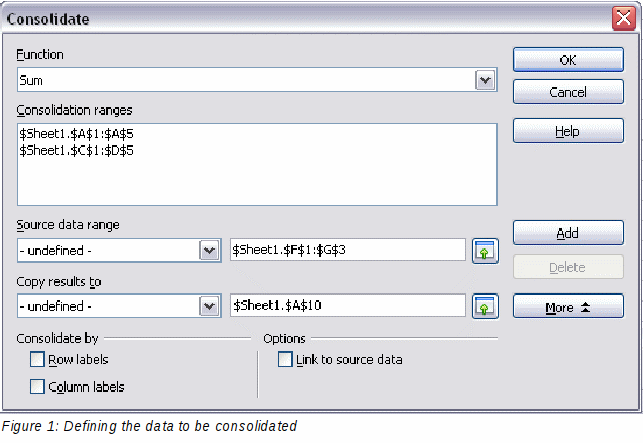
9. Select a function from the Function list. This specifies how the values of the consolidation ranges will be calculated. The default setting is Sum, which adds the corresponding cell values of the Source data range and gives the result in the target range.

Most of the available functions are statistical (such as Average, Min, Max, Stdev), and the tool is most useful when you are working with the same data over and over.

10. At this point you can click More in the Consolidate dialog to access the following additional settings:

• Select Link to source data to insert the formulas that generate the results into the target range, rather than the actual results. If you link the data, any values modified in the source range are automatically updated in the target range.

  Caution

  The corresponding cell references in the target range are inserted in consecutive rows, which are automatically ordered and then hidden from view. Only the final result, based on the selected function, is displayed.

• Under Consolidate by, select either Row labels or Column labels if the cells of the source data range are not to be consolidated corresponding to the identical position of the cell in the range, but instead according to a matching row label or column label. To consolidate by row labels or column labels, the label must be contained in the selected source ranges. The text in the labels must be identical, so that rows or columns can be accurately matched. If the row or column label of one source data range does not match any that exist in other source data ranges, it is added to the target range as a new row or column.

11. Click OK to consolidate the ranges.

12. If you are continually working with the same range, then you probably want to use Data → Define Range to give it a name.

The consolidation ranges and target range are saved as part of the document. If you later open a document in which consolidation has been defined, this data is still available.

Creating subtotals

SUBTOTAL is a function listed under the Mathematical category when you use the Function Wizard (Insert → Function). Because of its usefulness, the function has a graphical interface accessible from Data → Subtotals.

As the name suggests, SUBTOTAL totals data arranged in an array—that is, a group of cells with labels for columns. Using the Subtotals dialog, you can select up to three arrays, then choose a statistical function to apply to them. When you click OK, Calc adds subtotal and grand total rows to the selected arrays, using the Result and Result2 cell styles to differentiate those entries. By default, matching items throughout your array will be gathered together as a single group above a subtotal.

To insert subtotal values into a sheet:

1. Ensure that the columns have labels.

2. Select the range of cells that you want to calculate subtotals for, and then choose Data → Subtotals.

3. In the Subtotals dialog (Figure 2), in the Group by list, select the column by which the subtotals need to be grouped. A subtotal will be calculated for each distinct value in this column.

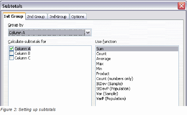
4. In the Calculate subtotals for box, select the columns containing the values that you want to create subtotals for. If the contents of the selected columns change later, the subtotals are automatically recalculated.

5. In the Use function box, select the function that you want to use to calculate the subtotals.

6. Click OK.

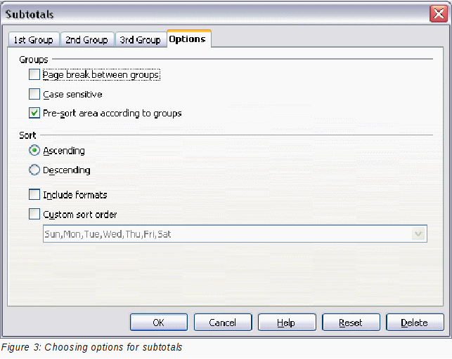
If you use more than one group, then you can also arrange the subtotals according to choices made on the dialog’s Options page (Figure 3), including ascending and descending order or using one of the predefined custom sorts defined in Tools → Options → LibreOffice Calc → Sort Lists.

Using “what if” scenarios

Scenarios are a tool to test “what-if” questions. Each scenario is named, and can be edited and formatted separately. When you print the spreadsheet, only the contents of the currently active scenario are printed.

A scenario is essentially a saved set of cell values for your calculations. You can easily switch between these sets using the Navigator or a drop-down list which can be shown beside the changing cells. For example, if you wanted to calculate the effect of different interest rates on an investment, you could add a scenario for each interest rate, and quickly view the results. Formulas that rely on the values changed by your scenario are updated when the scenario is opened. If all your sources of income used scenarios, you could efficiently build a complex model of your possible income.

Creating scenarios

Tools → Scenarios opens a dialog with options for creating a scenario.

To create a new scenario:

1. Select the cells that contain the values that will change between scenarios. To select multiple ranges, hold down the Ctrl key as you click. You must select at least two cells.

2. Choose Tools → Scenarios.

3. On the Create Scenario dialog (Figure 4), enter a name for the new scenario. It’s best to use a name that clearly identifies the scenario, not the default name as shown in the illustration. This name is displayed in the Navigator and in the title bar of the border around the scenario on the sheet itself.

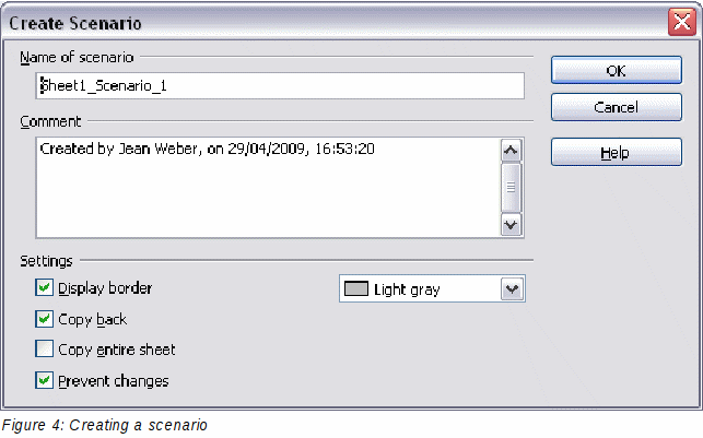
4. Optionally add some information to the Comment box. The example shows the default comment. This information is displayed in the Navigator when you click the Scenarios icon and select the desired scenario.

5. Optionally select or deselect the options in the Settings section. See page 8 for more information about these options.

6. Click OK to close the dialog. The new scenario is automatically activated.

You can create several scenarios for any given range of cells.

Settings

The lower portion of the Create Scenario dialog contains several options. The default settings (as shown in Figure 4) are likely to be suitable in most situations.

Display border

Places a border around the range of cells that your scenario alters. To choose the color of the border, use the field to the right of this option. The border has a title bar displaying the name of the active scenario. Click the arrow button to the right of the scenario name to open a drop-down list of all the scenarios that have been defined for the cells within the border. You can choose any of the scenarios from this list at any time.

Copy back

Copies any changes you make to the values of scenario cells back into the active scenario. If you do not select this option, the saved scenario values are never changed when you make changes. The actual behavior of the Copy back setting depends on the cell protection, the sheet protection, and the Prevent changes setting (see Table 1 on page 9).

Copy entire sheet

Adds to your document a sheet that permanently displays the new scenario in full. This is in addition to creating the scenario and making it selectable on the original sheet as normal.

Prevent changes

Prevents changes to a Copy back-enabled scenario when the sheet is protected but the cells are not. Also prevents changes to the settings described in this section while the sheet is protected. A fuller explanation of the effect this option has in different situations is given below.

Changing scenarios

Scenarios have two aspects that can be altered independently:

• Scenario properties (the settings described above)

• Scenario cell values (the entries within the scenario border)

The extent to which either of these aspects can be changed is dependent upon both the existing properties of the scenario and the current protection state of the sheet and cells.

Changing scenario properties

If the sheet is protected (Tools → Protect Document → Sheet), and Prevent changes is selected then scenario properties cannot be changed.

If the sheet is protected, and Prevent changes is not selected, then all scenario properties can be changed except Prevent changes and Copy entire sheet, which are disabled.

If the sheet is not protected, then Prevent changes does not have any effect, and all scenario properties can be changed.

Changing scenario cell values

Table 1 summarizes the interaction of various settings in preventing or allowing changes in scenario cell values.

Table 1: Prevent changes behavior for scenario cell value changes

Working with scenarios using the Navigator

After scenarios are added to a spreadsheet, you can jump to a particular scenario by selecting it from the list in the Navigator.

Click the Scenarios icon in the Navigator (see Figure 5). The defined scenarios are listed, along with the comments that were entered when the scenarios were created.

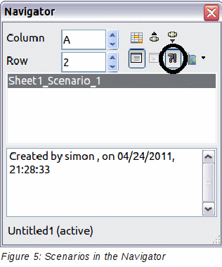
To apply a scenario to the current sheet, double-click the scenario name in the Navigator.

To delete a scenario, right-click the name in the Navigator and choose Delete.

To edit a scenario, including its name and comments, right-click the name in the Navigator and choose Properties. The Edit Properties dialog is the same as the Create Scenario dialog (Figure 4).

Tracking values in scenarios

To learn which values in the scenario affect other values, choose Tools → Detective → Trace Dependents. Arrows point to the cells that are directly dependent on the current cell.

Using other “what if” tools

Like scenarios, Data → Multiple Operations is a planning tool for “what if” questions. Unlike a scenario, the Multiple Operations tool does not present the alternate versions in the same cells or with a drop-down list. Instead, the Multiple Operations tool creates a formula array: a separate set of cells showing the results of applying the formula to a list of alternative values for the variables used by the formula. Although this tool is not listed among the functions, it is really a function that acts on other functions, allowing you to calculate different results without having to enter and run them separately.

To use the Multiple Operations tool, you need two arrays of cells. The first array contains the original or default values and the formulas applied to them. The formulas must be in a range.

The second array is the formula array. It is created by entering a list of alternative values for one or two of the original values.

Once the alternative values are created, you use the Multiple Operations tool to specify which formulas you are using, as well as the original values used by the formulas. The second array is then filled with the results of using each alternative value in place of the original values.

The Multiple Operations tool can use any number of formulas, but only one or two variables. With one variable, the formula array of alternative values for the variables will be in a single column or row. With two variables, you should outline a table of cells such that the alternative values for one variable are arranged as column headings, and the alternative values for the other variable act as row headings.

Setting up multiple operations can be confusing at first. For example, when using two variables, you need to select them carefully, so that they form a meaningful table. Not every pair of variables is useful to add to the same formula array. Yet, even when working with a single variable, a new user can easily make mistakes or forget the relationships between cells in the original array and cells in the formula array. In these situations, Tools → Detective can help to clarify the relations.

You can also make formula arrays easier to work with if you apply some simple design logic. Place the original and the formula array close together on the same sheet, and use labels for the rows and columns in both. These small exercises in organizational design make working with the formula array much less painful, particularly when you are correcting mistakes or adjusting results.

Multiple operations in columns or rows

In your spreadsheet, enter a formula to calculate a result from values that are stored in other cells. Then, set up a cell range containing a list of alternatives for one of the values used in the formula. The Multiple Operations command produces a list of results adjacent to your alternative values by running the formula against each of these alternatives.

In the Formulas field of the Multiple Operations dialog, enter the cell reference to the formula that you wish to use.

The arrangement of your alternative values dictates how you should complete the rest of the dialog. If you have listed them in a single column, you should complete the field for Column input cell. If they are along a single row, complete the Row input cell field. You may also use both in more advanced cases. Both single and double-variable versions are explained below.

The above can be explained best by examples. Cell references correspond to those in the following figures.

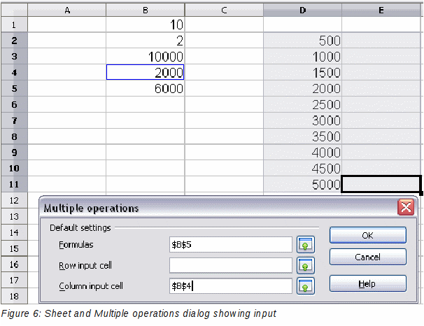
Let’s say you produce toys that you sell for $10 each (cell B1). Each toy costs $2 to make (cell B2), in addition to which you have fixed costs of $10,000 per year (cell B3). How much profit will you make in a year if you sell a particular number of toys?

Calculating with one formula and one variable

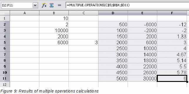
1. To calculate the profit, first enter any number as the quantity (items sold); in this example, 2000 (cell B4). The profit is found from the formula Profit=Quantity * (Selling price – Direct costs) – Fixed costs. Enter this formula in B5: =B4*(B1-B2)-B3.

2. In column D enter a variety of alternative annual sales figures, one below the other; for example, 500 to 5000, in steps of 500.

3. Select the range D2:E11, and thus the values in column D and the empty cells (which will receive the results of the calculations) alongside in column E.

4. Choose Data → Multiple Operations.

5. With the cursor in the Formulas field of the Multiple operations dialog, click cell B5.

6. Set the cursor in the Column input cell field and click cell B4. This means that B4, the quantity, is the variable in the formula, which is to be replaced by the column of alternative values. Figure 6 shows the worksheet and the Multiple operations dialog.

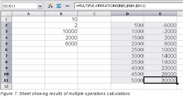
7. Click OK. The profits for the different quantities are now shown in column E. See Figure 7.

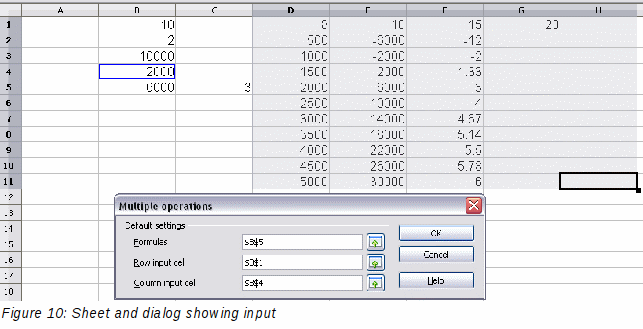
Calculating with several formulas simultaneously

1. In the sheet from the previous example, delete the contents of column E.

2. Enter the following formula in C5: =B5/B4. You are now calculating the annual profit per item sold.

3. Select the range D2:F11, thus three columns.

4. Choose Data → Multiple Operations.

5. With the cursor in the Formulas field of the Multiple operations dialog, select cells B5 and C5.

6. Set the cursor in the Column input cell field and click cell B4. Figure 8 shows the worksheet and the Multiple operations dialog.

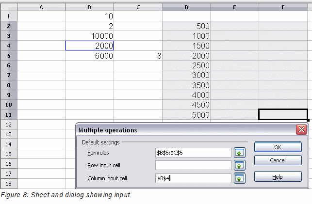
7. Click OK. Now the profits are listed in column E and the annual profit per item in column F.

Multiple operations across rows and columns

You can carry out multiple operations simultaneously for both columns and rows in so-called cross-tables. The formula must use at least two variables, the alternative values for which should be arranged so that one set is along a single row and the other set appears in a single column. These two sets of alternative values will form column and row headings for the results table produced by the Multiple Operations procedure.

Select the range defined by both data ranges (thus including all of the blank cells that are to contain the results) and choose Data → Multiple operations. Enter the cell reference to the formula in the Formulas field. The Row input cell and the Column input cell fields are used to enter the reference to the corresponding cells of the formula.

Calculating with two variables

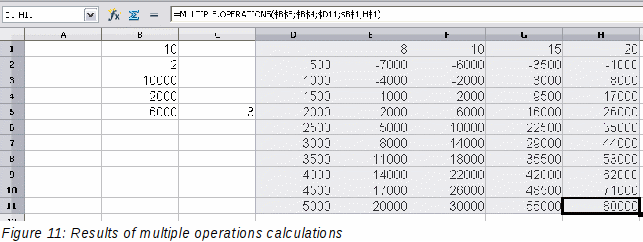
You now want to vary not just the quantity produced annually, but also the selling price, and you are interested in the profit in each case.

Expand the table shown in Figure 8. D2 thru D11 already contain the numbers 500, 1000 and so on, up to 5000. In E1 through H1 enter the numbers 8, 10, 15 and 20.

1. Select the range D1:H11.

2. Choose Data → Multiple Operations.

3. With the cursor in the Formulas field of the Multiple operations dialog, click cell B5 (profit).

4. Set the cursor in the Row input cell field and click cell B1. This means that B1, the selling price, is the horizontally entered variable (with the values 8, 10, 15 and 20).

5. Set the cursor in the Column input cell field and click cell B4. This means that B4, the quantity, is the vertically entered variable.

6. Click OK. The profits for the different selling prices are now shown in the range E2:H11.

Working backwards using Goal Seek

Usually, you create a formula to calculate a result based upon existing values. By contrast, using Tools → Goal Seek you can discover what values will produce the result that you want.

To take a simple example, imagine that the Chief Financial Officer of a company is developing sales projections for each quarter of the forthcoming year. She knows what the company’s total income must be for the year to satisfy stockholders. She also has a good idea of the company’s income in the first three quarters, because of the contracts that are already signed. For the fourth quarter, however, no definite income is available. So how much must the company earn in Q4 to reach its goal? The CFO can enter the projected earnings for each of the other three quarters along with a formula that totals all four quarters. Then she runs a goal seek on the empty cell for Q4 sales, and receives her answer.

Other uses of goal seek may be more complicated, but the method remains the same. Only one argument can be altered in a single goal seek.

Goal Seek example

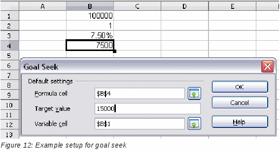
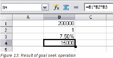
To calculate annual interest (I), create a table with the values for the capital (C), number of years (n), and interest rate (i). The formula is I = C*n*i.

Let us assume that the interest rate i of 7.5% and the number of years n (1) will remain constant. However, you want to know how much the investment capital C would have to be modified in order to attain a particular return I. For this example, calculate how much capital C would be required if you want an annual return of $15,000.

Enter each of the values mentioned above into adjacent cells (for Capital, C, an arbitrary value like $100,000 or it can be left blank; for number of years, n, 1; for interest rate, i, 7.5%). Enter the formula to calculate the interest, I, in another cell. Instead of C, n, and i, use the reference to the cell with the corresponding value. In our example (Figure 12), this would be =B1*B2*B3.

1. Place the cursor in the formula cell (B4), and choose Tools → Goal Seek.

2. In the Goal Seek dialog, the correct cell is already entered in the Formula cell field.

3. Place the cursor in the Variable cell field. In the sheet, click in the cell that contains the value to be changed, in this example it is B1.

4. Enter the desired result of the formula in the Target value field. In this example, the value is 15000. Figure 12 shows the cells and fields.

5. Click OK. A dialog appears informing you that the Goal Seek was successful. Click Yes to enter the goal value into the variable cell. The result is shown below.

Using the Solver

Tools → Solver amounts to a more elaborate form of Goal Seek. The difference is that the Solver deals with equations with multiple unknown variables. It is specifically designed to minimize or maximize the result according to a set of rules that you define.

Each of these rules defines whether an argument in the formula should be greater than, less than, or equal to the figure you enter. If you want the argument to remain unchanged, you must enter a rule that specifically states that the cell should be equal to its current entry. For arguments that you would like to change, you need to add two rules to define a range of possible values: the limiting conditions. For example, you can set the constraint that one of the variables or cells must not be bigger than another variable, or not bigger than a given value. You can also define the constraint that one or more variables must be integers (values without decimals), or binary values (where only 0 and 1 are allowed).

Once you have finished setting up the rules, click the Solve button to begin the automatic process of adjusting values and calculating results. Depending on the complexity of the task, this may take some time.

Solver example

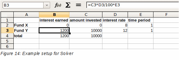
Let’s say you have $10,000 that you want to invest in two mutual funds for one year. Fund X is a low risk fund with 8% interest rate and Fund Y is a higher risk fund with 12% interest rate. How much money should be invested in each fund to earn a total interest of $1000?

To find the answer using Solver:

1. Enter labels and data:

• Row labels: Fund X, Fund Y, and total, in cells A2 thru A4.

• Column labels: interest earned, amount invested, interest rate, and time period, in cells B1 thru E1.

• Interest rates: 8 and 12, in cells D2 and D3.

• Time period: 1, in cells E2 and E3.

• Total amount invested: 10000, in cell C4.

2. Enter an arbitrary value (0 or leave blank) in cell C2 as amount invested in Fund X.

3. Enter formulas:

• In cell C3, enter the formula C4–C2 (total amount – amount invested in Fund X) as the amount invested in Fund Y.

• In cells B2 and B3, enter the formula for calculating the interest earned (see Figure 14).

• In cell B4, enter the formula B2+B3 as the total interest earned.

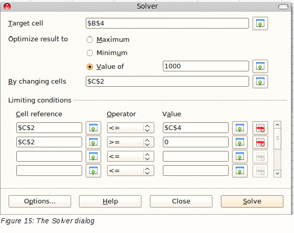
4. Choose Tools → Solver. The Solver dialog (Figure 15) opens.

5. Click in the Target cell field. In the sheet, click in the cell that contains the target value. In this example it is cell B4 containing total interest value.

6. Select Value of and enter 1000 in the field next to it. In this example, the target cell value is 1000 because your target is a total interest earned of $1000. Select Maximum or Minimum if the target cell value needs to be one of those extremes.

7. Click in the By changing cells field and click on cell C2 in the sheet. In this example, you need to find the amount invested in Fund X (cell C2).

8. Enter limiting conditions for the variables by selecting the Cell reference, Operator and Value fields. In this example, the amount invested in Fund X (cell C2) should not be greater than the total amount available (cell C4) and should not be less than 0.

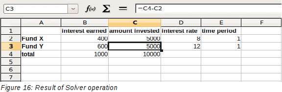
9. Click OK. A dialog appears informing you that the Solving successfully finished. Click Keep Result to enter the result in the cell with the variable value. The result is shown in Figure 16.