
Impress Guide
Chapter
7
Including Spreadsheets, Charts, and
Other Objects
This document is Copyright © 2005–2011 by its contributors as listed below. You may distribute it and/or modify it under the terms of either the GNU General Public License (http://www.gnu.org/licenses/gpl.html), version 3 or later, or the Creative Commons Attribution License (http://creativecommons.org/licenses/by/3.0/), version 3.0 or later.
All trademarks within this guide belong to their legitimate owners.
Contributors
Michele
Zarri
T. Elliot Turner
Jean Hollis Weber
Feedback
Please direct any comments or suggestions about this document to: documentation@global.libreoffice.org
Acknowledgments
This chapter is based on Chapter 7 of the OpenOffice.org 3.3 Impress Guide. The contributors to that chapter are:
Peter
Hillier-Brook Hazel Russman Jean Hollis Weber
Claire Wood Michele
Zarri
Publication date and software version
Published 31 July 2011. Based on LibreOffice 3.3.3.
Some keystrokes and menu items are different on a Mac from those used in Windows and Linux. The table below gives some common substitutions for the instructions in this chapter. For a more detailed list, see the application Help.
|
Windows/Linux |
Mac equivalent |
Effect |
|
Tools > Options menu selection |
LibreOffice > Preferences |
Access setup options |
|
Right-click |
Control+click |
Open context menu |
|
Ctrl (Control) |
z (Command) |
Used with other keys |
|
F5 |
Shift+z+F5 |
Open the Navigator |
|
F11 |
z+T |
Open Styles and Formatting window |
Contents
Using spreadsheets in Impress 4
Inserting a spreadsheet from a file 4
Inserting a blank spreadsheet 4
Resizing and moving a spreadsheet 6
How a spreadsheet is organized 6
Formatting spreadsheet cells 7
Opening a chart data window 12
Adding or removing elements from a chart 13
Resizing and moving the chart 15
Changing the chart area background 15
A spreadsheet embedded in Impress includes most of the functionality of a spreadsheet in Calc and is therefore capable of performing complex calculations and data analysis. However, if you plan to use complex data or formulas, you are better off performing the necessary operations in a separate Calc spreadsheet and use Impress only to display the embedded spreadsheet with the results.
You may also be tempted to use spreadsheets in Impress for creating complex tables or presenting data in a tabular format. However, the Table Design feature (described in Chapter 3) is often more suitable and faster.
To include spreadsheet cells in an Impress slide, you can either insert an existing file or insert a new table.
Inserting a spreadsheet from a file
When you insert an existing spreadsheet into your slide, subsequent changes that are made to the original spreadsheet file do not affect your slide. You can,however, make changes to the spreadsheet within your slide.
Go to the slide where you want to insert the spreadsheet.
Choose Insert > Object > OLE Object from the menu bar.
On the Insert OLE Object dialog box, choose Create from file . The dialog box changes to show a File field. Click Search.
On the Open dialog box, locate the file you want to insert, and then click OK.
Choose the Link to file option if you wish to insert the file as a live link.
The entire spreadsheet is inserted into your slide. If the spreadsheet contains more than one sheet and the one you want is not visible, double-click the spreadsheet and then select a different sheet from the row of sheet tabs at the bottom.
To add a blank spreadsheet to a slide:
Go to the slide where you want to insert the spreadsheet.
Choose Insert > Object > OLE Object from the menu bar.
On the Insert OLE Object dialog box, choose Create new and LibreOffice 3.3 Spreadsheet, then click OK.
This inserts a blank spreadsheet in the center of a slide, as shown in Figure 3. The spreadsheet is in edit mode, so you can insert data and modify the formatting. See “Entering data” and “Formatting spreadsheet cells” both on page 7.
When editing a spreadsheet, some of the items on the menu bar change, as does the Formatting toolbar (see Figure 4), to show entries and tools that support working with spreadsheets.
One of the most important changes is the presence of the Formula bar, just below the Formatting toolbar. The Formula bar contains (from left to right):
The active cell reference or the name of the selected range
The Formula Wizard button
The Sum and Formula buttons or the Cancel and Accept buttons (depending on the contents of the cell)
A long edit box to enter or review the contents of a cell
If you are familiar with Calc, you will immediately recognize the tools and the menu items since they are much the same.
Resizing and moving a spreadsheet
When resizing or moving a spreadsheet, ignore the first row and the first column (easily recognizable because of their light gray background) and the horizontal and vertical scroll bars). They are only used for editing purposes and will not be included in the visible area of the spreadsheet on the slide.
To resize the area occupied by the spreadsheet:
Double-click to enter edit mode, if it is not already active. Notice the black handles found in the gray border surrounding the spreadsheet (see Figure 3).
Move the mouse over one of the handles. The cursor changes shape to give a visual representation of the effects applied to the area.
Click and hold the left mouse button and drag the handle. The corner handles move the two adjacent sides simultaneously, while the handles at the midpoint of the sides modify one dimension at a time.
You can move the spreadsheet (change its position within the slide) whether in edit mode or not. In both cases:
Move the mouse over the border until the cursor changes to a four-headed arrow.
Click and hold the left mouse button and drag the spreadsheet to the desired position.
Release the mouse button.
When selected, the spreadsheet object is treated like any other object; therefore resizing it changes the scale rather than the spreadsheet area. This is not recommended, because it may distort the fonts and picture shapes.
How a spreadsheet is organized
A spreadsheet consists normally of multiple tables (called sheets) which in turn contain cells. However, in Impress only one of these tables can be shown at any given time on a slide.
The default for a spreadsheet embedded in Impress is one single table called Sheet 1. The name of the table is shown at the bottom of the spreadsheet area (see Figure 3).
If required, you can add other sheets. To do that:
Right-click on the bottom area near the existing tab.
Select Insert > Sheet from the pop-up menu.
Just as in Calc, you can rename a sheet or move it to a different position using the same pop-up menu or the Insert menu on the main menu bar.
|
Note |
Even if you have many sheets in your embedded spreadsheet, only one sheet—the one which is active when leaving the spreadsheet edit mode—is shown on the slide. |
Each of the sheets is further organized into cells. Cells are the elementary units of the spreadsheet. They are identified by a row number (shown on the left hand side on a gray background) and a column letter (shown in the top row also on a gray background). For example, the top left cell is identified as A1, while the third cell in the second row is C2. All data elements, whether text, numbers or formulas, are entered into a cell.
To move around the spreadsheet and select an active cell , you can:
Use the arrow keys.
Left-click with the mouse on the desired cell.
Use the combinations Enter and Shift+Enter to move one cell down or one cell up respectively; Tab key and Shift+Tab key to move one cell to the right or to the left respectively.
Other keyboard shortcuts are available to move quickly to certain cells of the spreadsheet. Refer to Chapter 5, Getting Started with Calc, in the Getting Started guide for further information.
Keyboard input is received by the active cell, identified by a thick black border (see Figure 3 where cell B3 is active). The cell reference (or coordinates) is also shown on the left hand end of the formula bar.
To insert data, first select the cell to make it active, then start typing . Note that the input is also added to the main part of the formula bar where it may be easier to read.
Impress
will try to automatically recognize the type of contents (text,
number, date, time, and so on) of a cell and apply default formatting
to it. Note how the formula bar icons change according to the type of
input, displaying Accept and Reject buttons (![]() )
whenever the input is not a formula. Use the green Accept button to
confirm the input made in a cell or simply select a different cell.
In case Impress wrongly recognizes the type of input, you can change
it using the toolbar shown in Figure 4, or from Format
> Cells in the main menu bar.
)
whenever the input is not a formula. Use the green Accept button to
confirm the input made in a cell or simply select a different cell.
In case Impress wrongly recognizes the type of input, you can change
it using the toolbar shown in Figure 4, or from Format
> Cells in the main menu bar.
|
Tip |
Sometimes it is useful to treat numbers as text (for example, telephone numbers) and to prevent Impress from removing the leading zeros or right align them in a cell. To force Impress to treat the input as text, type a single apostrophe ' (U + 00B4) before entering the number. |
Often, for the purposes of a presentation, it may be necessary to increase the size of the font considerably or to match it to the style used in the presentation.
The fastest and most flexible way to format the embedded spreadsheet is to make use of styles. When working on an embedded spreadsheet, you can access the cell styles created in Calc and use them. However, a better approach is to create specific cell styles for presentation spreadsheets, as the Calc cell styles are likely to be unsuitable when working within Impress.
To apply a style to a cell or group of cells simultaneously (or manually format their cell attributes), first select the range to which the changes will apply. A range consists of one or more cells, normally forming a rectangular area. A selected range consisting of more than one cell can be recognized easily because all its cells are shaded. To select a multiple-cell range:
Click on the first cell belonging to the range (either the left top cell or the right bottom cell of the rectangular area).
Keep the left mouse button pressed and move the mouse to the opposite corner of the rectangular area which will form the selected range.
Release the mouse button.
To add further cells to the selection, hold down the Control key and repeat the steps 1 to 3 above.
|
Tip |
You can also click on the first cell in the range, hold down the Shift key, and click in the cell in the opposite corner. Refer to Chapter 5, Getting Started with Calc, in the Getting Started book for further information on selecting ranges of cells. |
Some shortcuts are very useful to speed up selection and are listed below:
To select the whole visible sheet, click on the blank cell between the row and column indexes, or press Control+A.
To select a column, click on the column index at the top of the spreadsheet.
To select a row, click on the row index on the left hand side of the spreadsheet.
Once the range is selected, you can modify the formatting, such as font size, alignment (including vertical alignment), font color, number formats, borders, background and so on. To access these settings, choose Format > Cells from the main menu bar (or right-click and choose Format Cells from the pop-up menu). This command opens the dialog box shown in Figure 5.
If the text does not fit the width of the cell, you can increase the width by hovering the mouse over the line separating two columns until the mouse cursor changes to a double-headed arrow; then click the left button and drag the separating line to the new position. A similar procedure can be used to modify the height of a cell (or group of cells).
To insert rows and columns in a spreadsheet, use the Insert menu or right-click on the row and column headers and select the appropriate option from the pop up menu. To merge multiple cells, select the cells to be merged and select Format > Merge cells from the main menu bar. To split a group of cells, select the group and deselect Format > Merge Cells (which will now have a checkmark next to it).
When you are satisfied with the formatting and the appearance of the table, exit edit mode by clicking outside the spreadsheet area. Note that Impress will display exactly the section of the spreadsheet that was on the screen before leaving edit mode. This allows you to hide additional data from view, but it may cause the apparent loss of rows and columns. Therefore, take care that the desired part of the spreadsheet is showing on the screen before leaving edit mode.
|
Tip |
To get back into edit mode, right click and select Edit. |
The use of charts is described in detail in Chapter 3, Creating Charts and Graphs, of the Calc Guide.
To add a chart to a slide:
Select the Insert
Chart icon on the slide layout (see Figure 6) or
use Insert
> Chart, or
click the Insert
Chart icon
![]() on the Standard toolbar.
on the Standard toolbar.
A full-sized chart appears; it contains arbitrary sample data (see Figure 7).
To enter your own data in the chart, see “Entering chart data” on page 12.
Your data can be presented using a variety of different charts; choose a chart type that best suits the message you want to convey to your audience (see “Chart types” on page 11).
To choose a chart type:
Double-click the sample chart. The window changes; the side panes are gone and the main toolbar shows tools specific for charts. The chart itself now has a gray border. (If the main toolbar is not showing, select View > Toolbars > Main Toolbar.)
Click the Chart
Type icon
![]() or select Format
>
Chart Type, or right-click on the chart and choose
Chart
Type. The Chart Type dialog
box appears.
or select Format
>
Chart Type, or right-click on the chart and choose
Chart
Type. The Chart Type dialog
box appears.
As you change selections in the left-hand list, the chart examples on the right, and the chart in the main window, both change. If you move the Chart Type dialog box to one side, you can see the full effect in the main window.
As you change chart types, other selections become available on the right-hand side. For example, some chart types have both three-dimensional and two-dimensional variants; 3D charts have further choices of shape for the columns or bars.
Choose the chart characteristics you want, and then click OK. The Chart Type dialog box closes and you return to the edit window.
Now you can continue to format the chart, add data to the chart, or click outside the chart to return to normal view.
The following summary of the chart types available will help you choose a type suitable for your data. For more detail, see Chapter 3, Creating Charts and Graphs, in the Calc Guide.
Column charts
Column charts are commonly used for data that shows trends over time. They are best for charts that have a relatively small number of data points. (For large time series, a line chart would be better.) This is the default chart type.
Bar charts
Bar charts are excellent for giving an immediate visual impact for data comparison where time is not important, such as comparing the popularity of a few products in a marketplace.
Pie charts
Pie charts are excellent when you need to compare proportions, for example, comparisons of departmental spending: what the department spent on different items or what different departments spent. They work best with smaller numbers of values, about half a dozen; more than this and the visual impact begins to fade.
This is one of the charts that can be made into a 3D chart. It can then be tilted, given shadows, and generally turned into a work of art. You can choose to explode the pie chart, but this is an all or nothing option, giving you no control over the degree of separation of the segments.
Area charts
An area chart is a version of a line or column graph. It may be useful where you wish to emphasize volume of change. Area charts have a greater visual impact than a line chart, but the data you use will make a difference. You may need to use transparency values in an area chart.
Line charts
A line chart is a time series with a progression. It is ideal for raw data, and useful for charts with plentiful data showing trends or changes over time, where you want to emphasize continuity. On line charts, the x-axis is ideal for representing time series data. 3D lines confuse the viewer, so just using a thicker line often works better.
Scatter or XY charts
Scatter charts are great for visualizing data that you have not had time to analyze, and they may be the best for data when you have a constant value for comparison: for example weather data, reactions under different acidity levels, conditions at altitude, or any data which matches two numeric series. The x-axis usually plots the independent variable or control parameter (often a time series).
Bubble charts
A bubble chart is used to represent three variables: two identify the position of the center of a bubble on a Cartesian graph, while the third variable indicates the radius of the bubble.
Net charts
A net chart is similar to polar or radar graphs. They are useful for comparing data that are not time series, but show different circumstances, such as variables in a scientific experiment. The poles of the net chart are the y-axes of other charts. Generally, between three and eight axes are best; any more and this type of chart becomes confusing.
Stock charts
A stock chart is a specialized column graph specifically for stocks and shares. You can choose traditional lines, candlestick, and two-column charts. The data required for these charts is quite specialized, with series for opening price, closing price, and high and low prices. The x-axis represents a time series.
Column and line charts
A column and line chart is a combination of two other chart types. It is useful for combining two distinct but related data series, for example sales over time (column) and the profit margin trends (line).
If the chart is not already in edit mode (with a gray border), double-click it. The main toolbar now shows tools specifically for charts. (If the main toolbar is not showing, select View > Toolbars > Main Toolbar.)
Click the Chart
Data icon
![]() or select View
>
Chart Data Table, or right-click on the chart and
choose Chart
Data Table. The Data Table dialog
box (Figure 9) appears.
or select View
>
Chart Data Table, or right-click on the chart and
choose Chart
Data Table. The Data Table dialog
box (Figure 9) appears.
|
Tip |
If you drag the Data Table dialog box so that your chart is visible, you can then immediately see the results of each change after clicking in a different cell. |
Enter data in the Data Table dialog box. Type or paste information into the boxes within the desired rows and columns.
You can use the buttons in the top left corner for large-scale editing:
The two Insert buttons insert a row or column (series).
The Delete buttons remove a selected row or column (series) with its data.
The Move buttons move the contents of the selected column to the right, or the contents of the selected row down.
Adding or removing elements from a chart
Figure 10: Chart Insert menu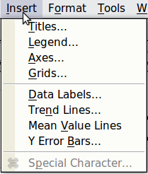
The default chart includes only
two elements: the chart wall and the legend (also known as the key).
You can add other elements using the Insert
menu (Figure 10). The various choices open dialog boxes in which you
can specify details.
The Format menu (Figure 11) has many options for formatting and fine-tuning the look of your charts.
Double-click the chart so that it is enclosed by a gray border indicating edit mode, then select the chart element that you want to format. Choose Format from the menu bar, or right-click to display a pop-up (context) menu relevant to the selected element.
The formatting choices are as follows:
Format Selection opens a dialog box in which you can specify the area fill, borders, transparency, characters, font effects, and position of the selected element of the chart.
Position and Size opens the Position and Size dialog box (see “Resizing and moving the chart”).
Arrangement provides two choices: Bring Forward and Send Backward, of which only one may be active for specific items. Use these choices to arrange overlapping data series.
Title formats the titles of the chart and its axes.
Legend formats the location, borders, background, and type of the legend.
Axis formats the lines that create the chart as well as the font of the text that appears on both the X and Y axes.
Grid formats the lines that create a grid for the chart.
Chart Wall, Chart Floor, and Chart Area are described in the following sections.
Chart Type changes what kind of chart is displayed and whether it is two- or three-dimensional.
3D View formats the various viewing angles of 3D chart.
|
Note |
Chart Floor and 3D View are available only for a 3D chart. These options are unavailable (grayed out) if a 2D chart is selected. |
A chart has two main areas: the chart wall and the chart area. These control different settings and attributes for the chart. Knowing the difference is helpful when formatting a chart.
Chart wall contains the graphic of the chart displaying the data.
Chart area is the area surrounding the chart graphic. The (optional) chart title and the legend (key) are in the chart area.
|
Note |
Format > Chart Floor is only available for 3D charts and has the same formatting options as Chart Area and Chart Wall. |
You can resize or move all elements of a chart at the same time, in two ways: interactively, or by using the Position and Size dialog box. You may wish to use a combination of both methods.
To resize a chart interactively:
Click on the chart to select it. Green sizing handles appear around the chart.
To increase or decrease the size of the chart, click and drag one of the corner handles. To maintain the correct aspect ratio, hold the Shift key down while you click and drag.
To move a chart interactively:
Click on the chart to select it. Green sizing handles appear around the chart.
Hover the mouse pointer anywhere over the chart other than on a handle. When it changes shape, click and drag the chart to its new location.
Release the mouse button when the element is in the desired position.
To resize or move a chart using the Position and Size dialog box:
Click on the chart to select it. Green sizing handles appear around the chart.
Choose Format > Position and Size from the menu bar, or right-click and choose Position and Size from the pop-up menu, or press F4. For more about the use of this dialog box, see Chapter 6, Formatting Graphic Objects.
You may wish to move or resize individual elements of a chart, independent of other chart elements. For example, you may wish to move the legend to a different place. Pie charts allow individual wedges of the pie to be moved (in addition to the choice of “exploding” the entire pie).
Double-click the chart so that is enclosed by a gray border.
Click any of the elements—the title, the legend, or the chart graphic—to select it. Green resizing handles appear.
Move the pointer over the selected element. When it changes shape, click and drag to move the element.
Release the mouse button when the element is in the desired position.
|
Note |
If your graphic is 3D, round red handles appear which control the three-dimensional angle of the graphic. You cannot resize or reposition the graphic while the round red handles are showing. Shift + Click to get back to the green resizing handles. You can now resize and reposition your 3D chart graphic. See the following tip. |
|
Tip |
You can resize the chart graphic using its green resizing handles (Shift + Click, then drag a corner handle to maintain the proportions). However, you cannot resize the title or the key. |
Changing the chart area background
The chart area is the area surrounding the chart graphic, including the (optional) main title and key.
Double-click the chart so that it is enclosed by a gray border.
Select Format > Chart Area.
In the Chart Area dialog box, choose the desired format settings.
Changing the chart graphic background
The chart wall is the area that contains the chart graphic.
Double-click the chart so that it is enclosed by a gray border.
Select Format > Chart Wall. The Chart Wall window appears. It has the same formatting options as described in “Changing the chart area background” above.
Choose your settings and click OK.
Impress offers the capability of inserting in a slide various types of objects such as music or video clips, Writer documents, Math formulas, generic OLE objects and so on. A typical presentation may contain movie clips, sound clips, OLE objects and formulas; other objects are less frequently used since they do not appear during a slide show.
This section covers the part of the Insert menu shown in Figure 14: Movie and Sound, and Object.
To insert a movie clip or a sound into a presentation:
Click the Insert Movie icon on the slide layout (see Figure 6) or choose Insert > Movie and Sound from the menu bar.
In the Insert Movie and Sound dialog box, select the media file to insert, and click Open to place the object on the slide.
|
Tip |
To see a list of audio and video file types supported by Impress, open the drop-down list of file types near the bottom of the Insert Movie and Sound dialog box. This list defaults to All movie and sound files, enabling you to choose an unsupported type such as .MOV. |
To insert media clips directly from the Gallery:
If the Gallery is not already open, choose Tools > Gallery from the menu bar.
Browse to the Theme containing media files (for example the Sounds theme).
Click on the movie or sound to be inserted and drag it into the slide area.
The Media Playback toolbar (Figure 15) is automatically opened (by default, at the bottom of the screen, just above the Drawing toolbar; it can also be made to float). You can preview the media object as well as resize it. If the toolbar does not open, select View > Media Playback.
The Media Playback toolbar contains the following tools:
Add button: opens a dialog box where you can select the media file to be inserted.
Play, Pause, Stop buttons: control the media playback.
Repeat button: if pressed, the media will restart when finished.
Playback slider: selects the position within the media clip.
Timer: displays the current position of the media clip.
Mute Button: when selected, the sound will be suppressed.
Volume Slider: adjusts the volume of the media clip.
Scaling drop-down menu: (only available for movies) allows scaling of the movie clip.
The movie will start playing as soon as the slide is shown during the presentation.
Note that Impress will only link the media clip, not embed it. Therefore if the presentation is moved to a different computer, the link will be broken and the media clip will not play. To prevent this from happening:
Place the media file which is to be included in the presentation in the same folder where the presentation is stored.
Insert the media file in the presentation.
Send both the presentation and the the media file to the computer which is to be used for the presentation and place both files in the same folder on that computer.
Impress offers the possibility to preview the media clips that are to be inserted by means of the embedded media player. To open it select Tools > Media Player. The media player is shown in Figure 16. Its toolbar is the same as that of the Media Playback toolbar described above.
Use an OLE (Object Linking and Embedding) object to insert in a presentation either a new document or an existing one. Embedding inserts a copy of the object and details of the presumed source program in the target document; this is the program which is associated with the file type by the operating system. The major benefit of an OLE object is that it is quick and easy to edit the contents just by double-clicking on it. You can also insert a link to the object that will appear as an icon rather than an area showing the contents itself.
To create and insert a new OLE object:
Select Insert > Object > OLE object from the main menu. This opens the dialog box shown in Figure 2 on page 5.
Select Create new and select the object type among the available options.
Click OK. An empty container is placed in the slide.
Double-click on the OLE object to enter the edit mode of the object. The application devoted to handling that type of file will open the object.
|
Note |
If the object inserted is handled by LibreOffice, then the transition to the program to manipulate the object will be seamless; in other cases the object opens in a new window and an option in the File menu becomes available to update the object you inserted. |
To insert an existing object:
Select Insert > Object > OLE object from the main menu.
In the Insert OLE Object dialog box, select Create from file. The dialog box changes to look like Figure 1 on page 4.
To insert the object as a link, select the Link to file option. Otherwise, the object will be embedded.
Click Search, select the required file in the file window, then click Open. A section of the inserted file is shown on the slide.
Under Windows, the Insert OLE Object dialog box has an extra entry, Further objects.
Double-click on the entry Further objects to open the dialog box shown in Figure 17.
Select Create New to insert a new object of the type selected in the Object Type list, or select Create from File to create a new object from a file.
If you choose Create from File, the dialog box shown in Figure 18 opens. Click Browse and choose the file to insert. The inserted file object is editable by the Windows program that created it.
If instead of inserting an object, you want to insert a link to an object, select the Display As Icon checkbox.
Use Insert > Object > Formula to create a Math object in a slide. When editing a formula, the main menu changes into the Math main menu.
Care should be taken about the font sizes used in order to make them compatible with the font size used in the rest of the slide. To change the font attributes of the Math object, select Format > Font Size from the main menu bar. To change the font type, select Format > Fonts from the main menu bar.
For additional information on how to create formulas, refer to Chapter 9, Getting Started with Math, in the Getting Started guide, or the Math Guide.
|
Note |
Unlike formulas in Writer, a formula in Impress is treated as an object; therefore it will not be automatically aligned with the rest of the text. The formula can be however moved around (but not resized) like any other object. |
Inserting the contents of a file
You can insert the contents of certain files into a presentation. The types of file accepted are LibreOffice Draw file, HTML files, or plain text files.
Select Insert > File from the main menu to open a file picker window. If there is an internet connection, it is also possible to insert a URL in the file name field. Select the file and click Insert.